Directory of Visualizations
Based on The R Graph Gallery


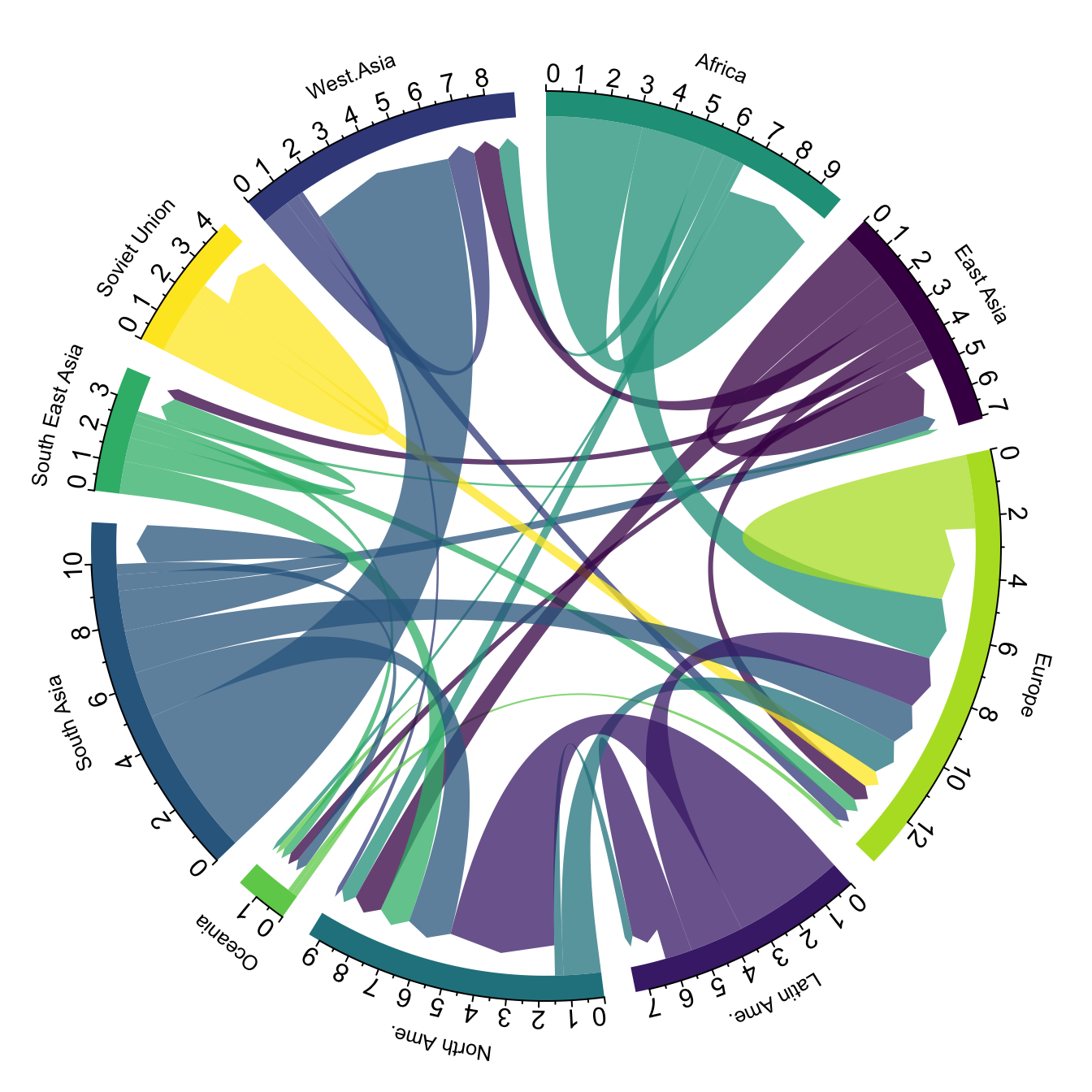
Flow


Chord diagram Network Sankey Arc diagram Edge bundling
- Visualization of interconnection between entities
- Generally, two datasets are required: nodes and edges
- Data wrangling is a bit different
Flow Network
library(ggraph)library(tidygraph)as_tbl_graph(highschool) |> mutate(Popularity = centrality_degree( mode="in")) |>ggraph(layout="kk") + geom_node_point( aes(size=Popularity)) + theme(legend.position="top")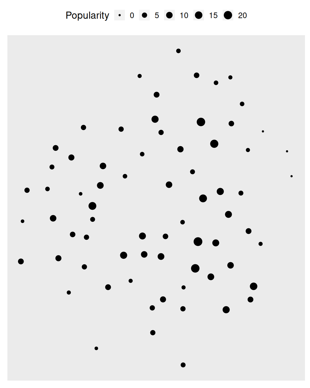
Flow Network
library(ggraph)library(tidygraph)as_tbl_graph(highschool) |> mutate(Popularity = centrality_degree( mode="in")) |>ggraph(layout="kk") + geom_node_point( aes(size=Popularity)) + geom_edge_link( arrow=arrow( length=unit(0.1, "inches"), type="closed")) + theme(legend.position="top")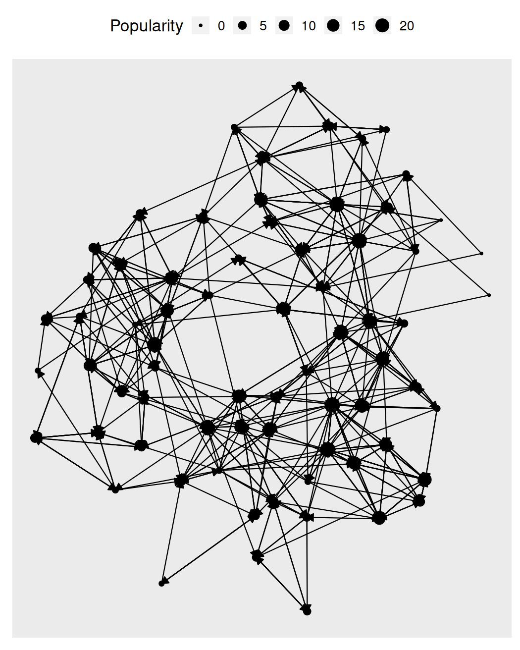
Flow Network
library(ggraph)library(tidygraph)as_tbl_graph(highschool) |> mutate(Popularity = centrality_degree( mode="in")) |>ggraph(layout="kk") + geom_node_point( aes(size=Popularity)) + geom_edge_fan( aes(alpha=after_stat(index)), show.legend=FALSE) + theme(legend.position="top")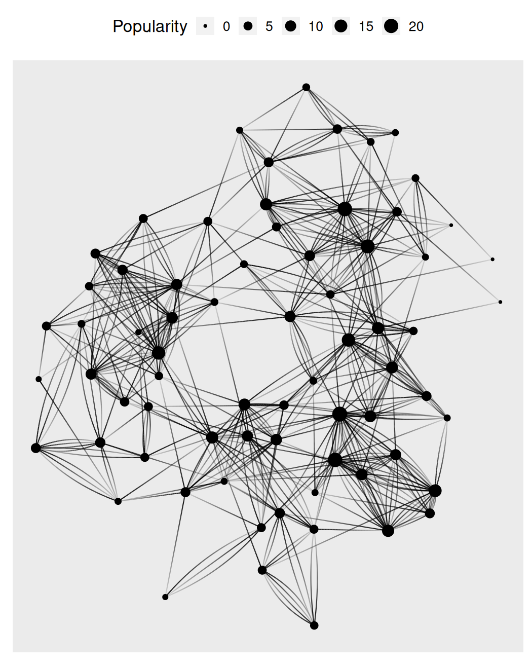
Flow Network
library(ggraph)library(tidygraph)as_tbl_graph(highschool) |> mutate(Popularity = centrality_degree( mode="in")) |>ggraph(layout="kk") + geom_node_point( aes(size=Popularity)) + geom_edge_fan( aes(alpha=after_stat(index), color=factor(year)), show.legend=FALSE) + theme(legend.position="top")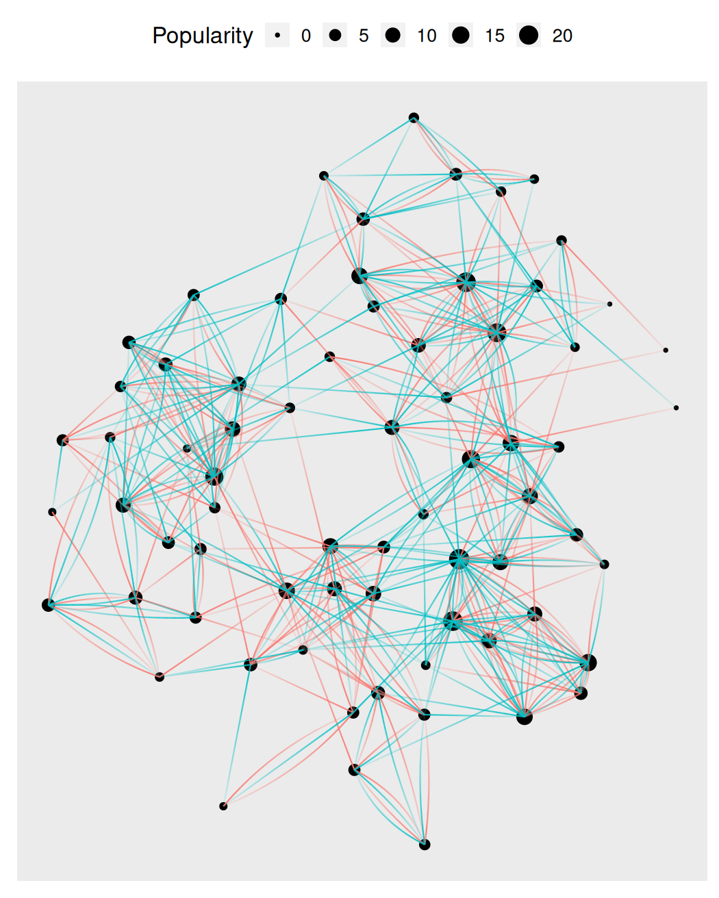
Flow Network
library(ggraph)library(tidygraph)as_tbl_graph(highschool) |> mutate(Popularity = centrality_degree( mode="in")) |>ggraph(layout="kk") + geom_node_point( aes(size=Popularity)) + geom_edge_fan( aes(alpha=after_stat(index)), show.legend=FALSE) + facet_edges(~year, ncol=1) + theme(legend.position="top")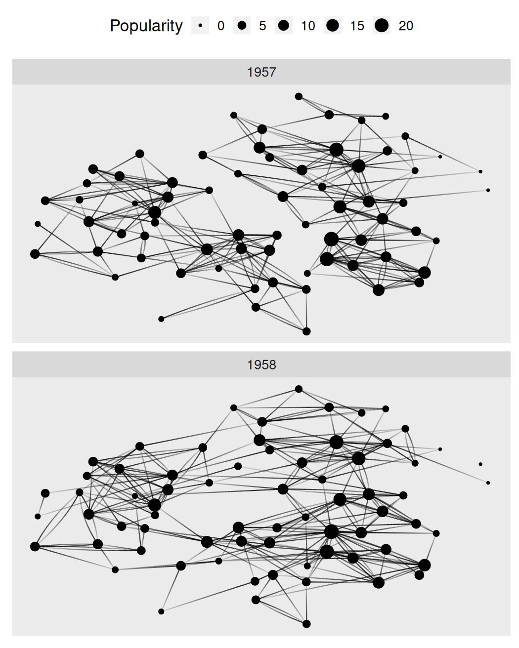
Flow Network
library(ggraph)library(tidygraph)as_tbl_graph(highschool) |> mutate(Popularity = centrality_degree( mode="in")) |>ggraph(layout="kk") + geom_node_point( aes(size=Popularity)) + geom_edge_fan( aes(alpha=after_stat(index)), show.legend=FALSE) + facet_edges(~year, ncol=1) + theme_graph(base_size=16, foreground="#a53253", fg_text_colour="white") + theme(legend.position="top")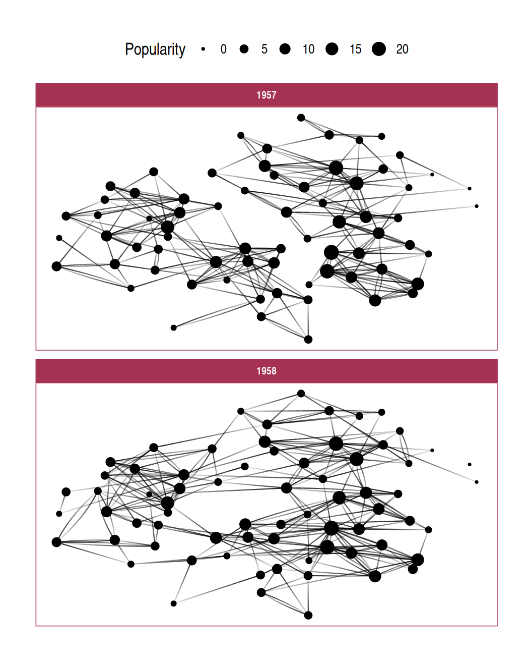
Flow Arc diagram
library(ggraph)library(tidygraph)as_tbl_graph(highschool) |> mutate(Popularity = centrality_degree( mode="in")) |>ggraph(layout="linear") + geom_node_point( aes(size=Popularity)) + geom_edge_arc( aes(alpha=after_stat(index)), show.legend=FALSE) + facet_edges(~year, ncol=1) + theme_graph(base_size=16, foreground="#a53253", fg_text_colour="white") + theme(legend.position="top")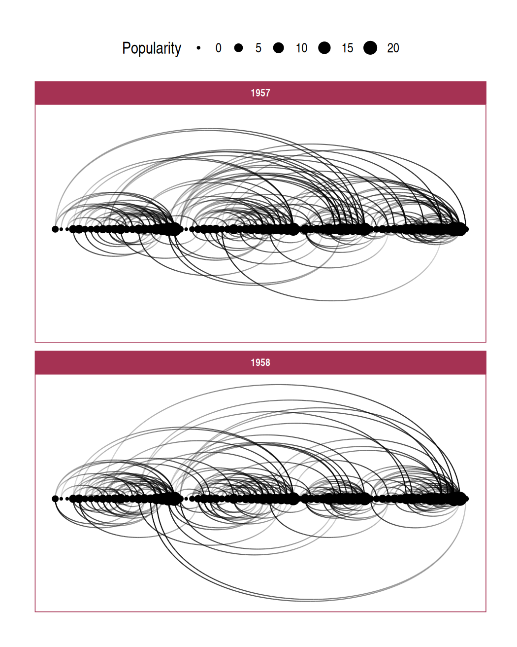
Flow Arc diagram
library(ggraph)library(tidygraph)as_tbl_graph(highschool) |> mutate(Popularity = centrality_degree( mode="in")) |>ggraph(layout="linear", circular=TRUE) + coord_fixed() + geom_node_point( aes(size=Popularity)) + geom_edge_arc( aes(alpha=after_stat(index)), show.legend=FALSE) + facet_edges(~year, ncol=1) + theme_graph(base_size=16, foreground="#a53253", fg_text_colour="white") + theme(legend.position="top")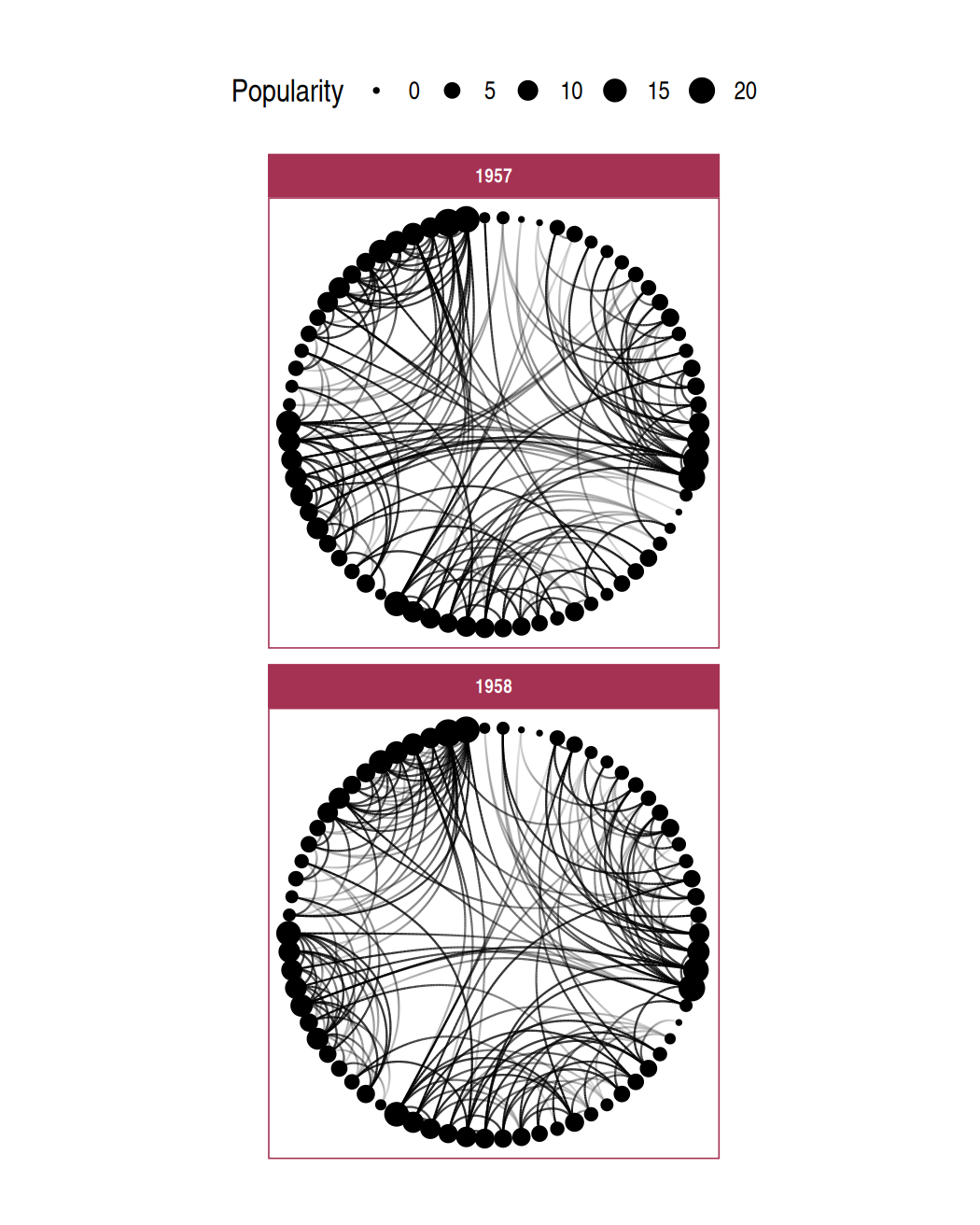
Flow Edge bundling
< Contents | Data from ggraph manual
library(ggraph)library(tidygraph)# flareGraph <- ...# importFrom <- ...# importTo <- ...ggraph(flareGraph, "dendrogram", circular=TRUE) + coord_fixed() + geom_node_point() + theme_graph(base_size=16)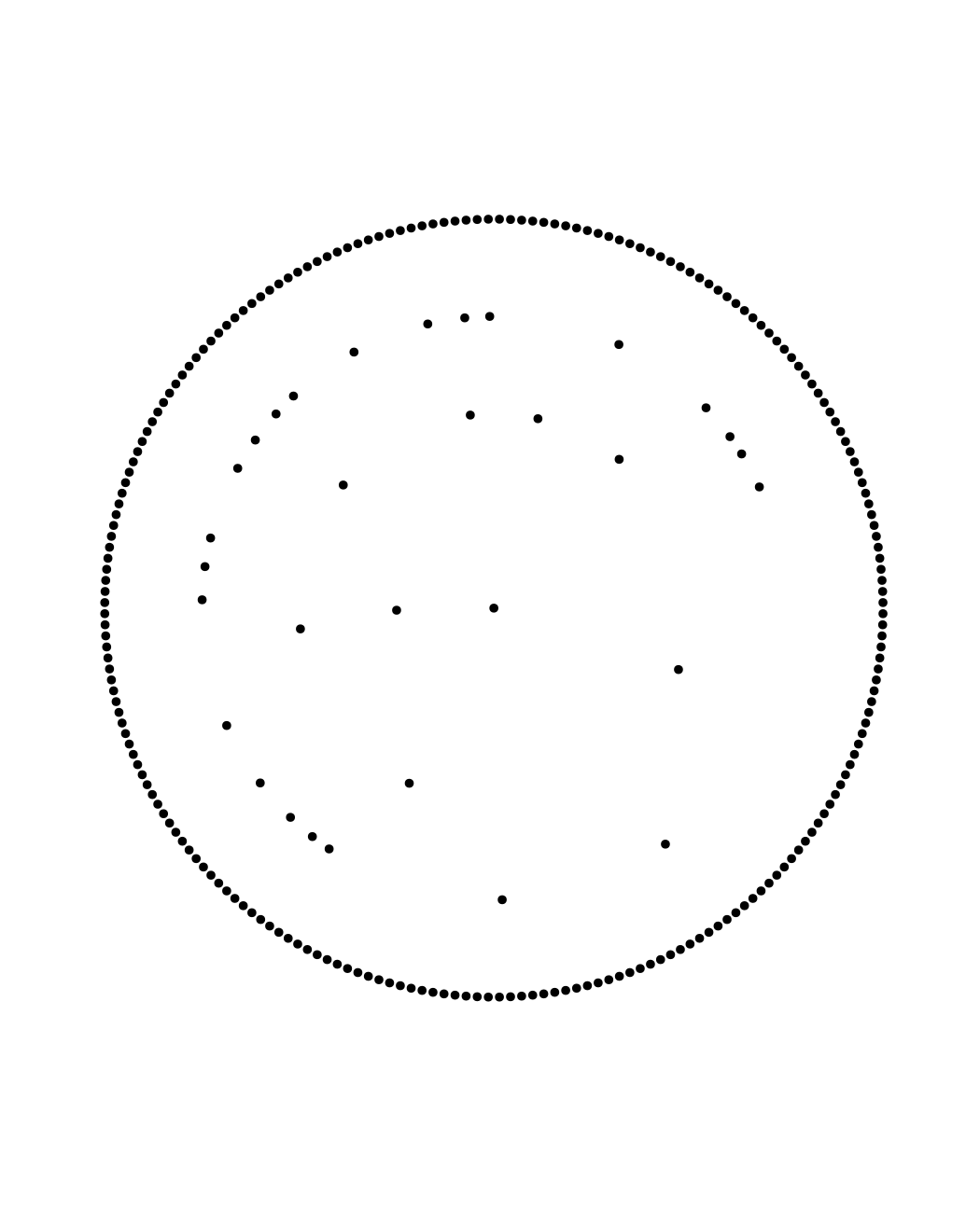
Flow Edge bundling
< Contents | Data from ggraph manual
library(ggraph)library(tidygraph)# flareGraph <- ...# importFrom <- ...# importTo <- ...ggraph(flareGraph, "dendrogram", circular=TRUE) + coord_fixed() + geom_node_point( aes(filter=leaf, color=class)) + theme_graph(base_size=16) + theme(legend.position="top")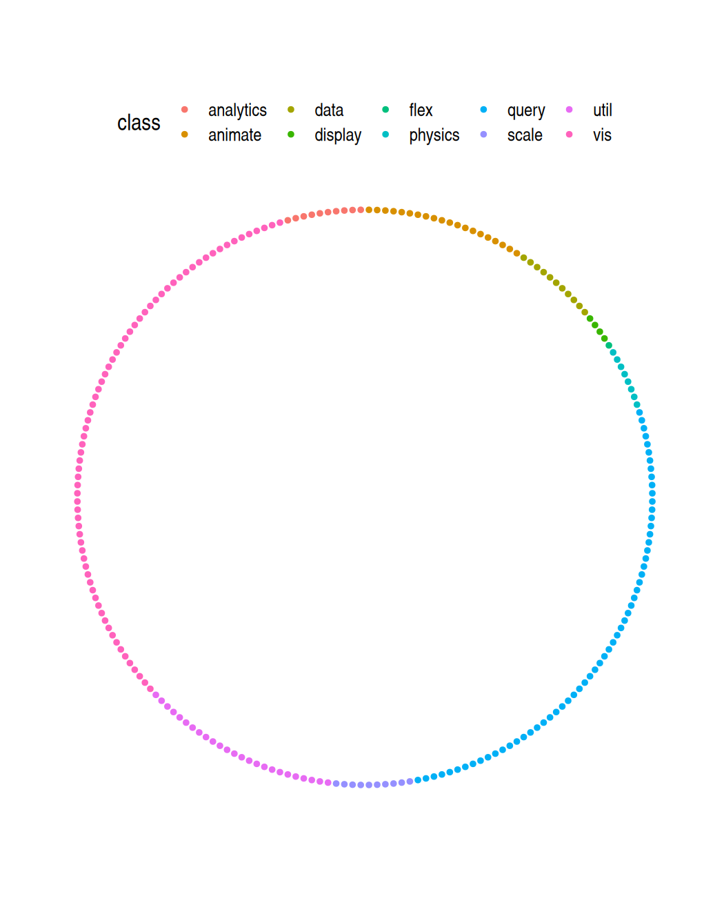
Flow Edge bundling
< Contents | Data from ggraph manual
library(ggraph)library(tidygraph)# flareGraph <- ...# importFrom <- ...# importTo <- ...ggraph(flareGraph, "dendrogram", circular=TRUE) + coord_fixed() + geom_node_point( aes(filter=leaf, color=class)) + geom_conn_bundle( aes(color=after_stat(index)), data=get_con(importFrom, importTo), edge_alpha=0.25) + theme_graph(base_size=16) + theme(legend.position="top")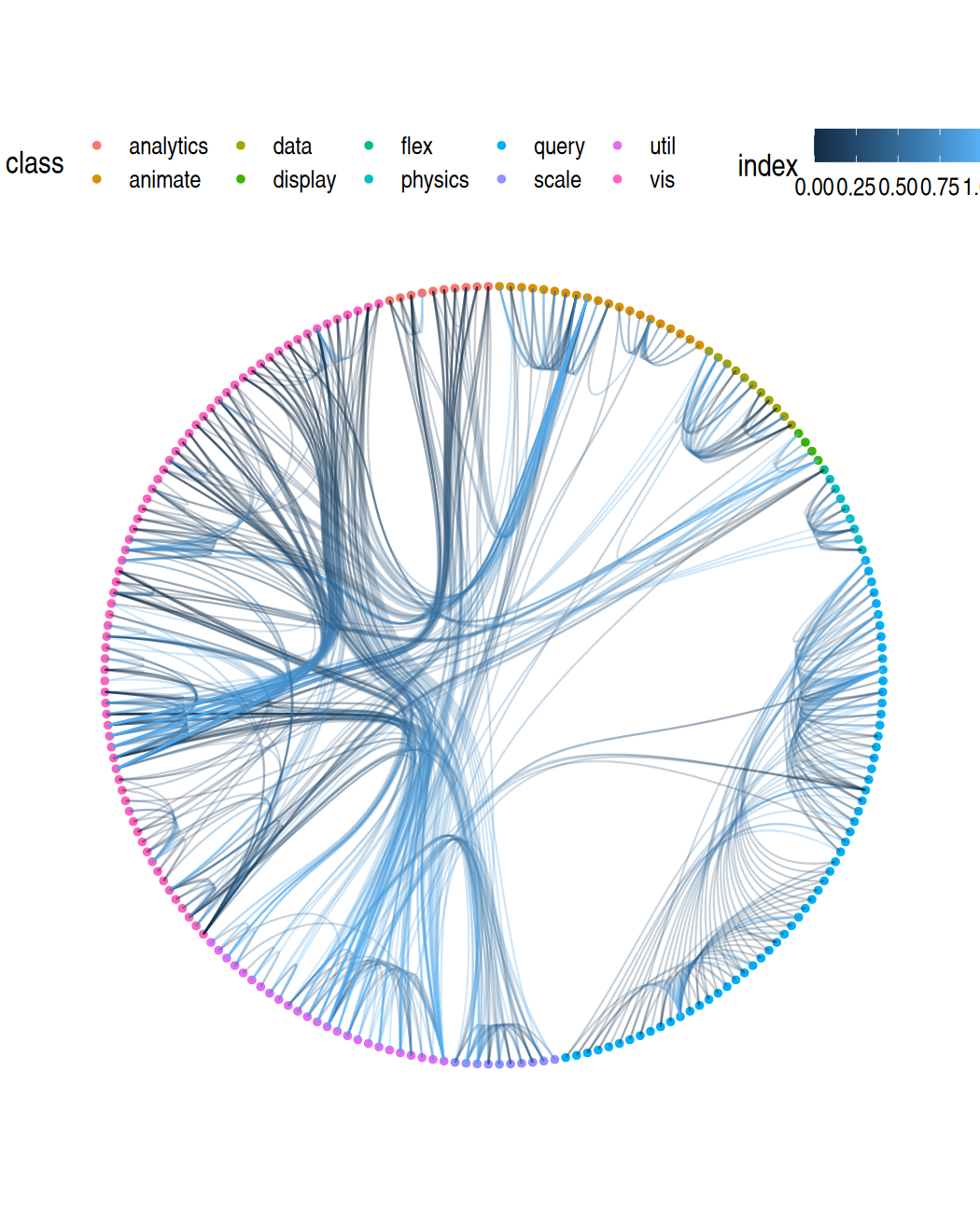
Flow Edge bundling
< Contents | Data from ggraph manual
library(ggraph)library(tidygraph)# flareGraph <- ...# importFrom <- ...# importTo <- ...ggraph(flareGraph, "dendrogram", circular=TRUE) + coord_fixed() + geom_node_point( aes(filter=leaf, color=class)) + geom_conn_bundle( aes(color=after_stat(index)), data=get_con(importFrom, importTo), edge_alpha=0.25) + scale_edge_colour_distiller( NULL, guide="edge_direction") + theme_graph(base_size=16) + theme(legend.position="top")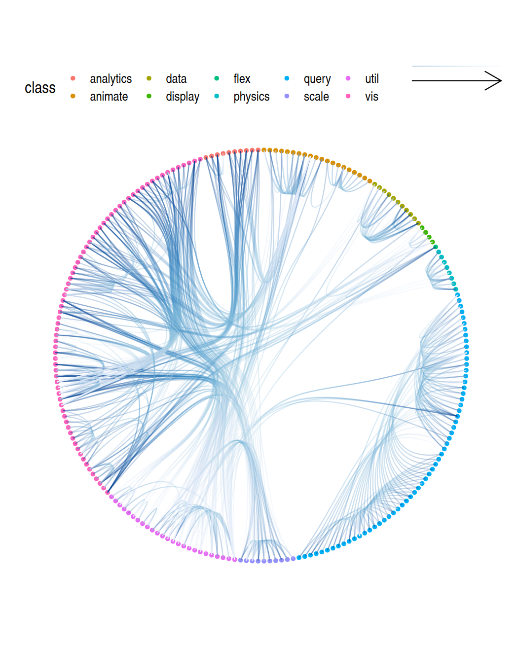
Flow Sankey / Alluvial
# remotes::install_github(# "davidsjoberg/ggsankey")df <- mtcars |> ggsankey::make_long( cyl, vs, am, gear, carb)ggplot(df) + aes(x, next_x=next_x, node=node, next_node=next_node, fill=factor(node)) + ggsankey::geom_sankey() + scale_fill_viridis_d() + labs(x=NULL) + theme(legend.position="top")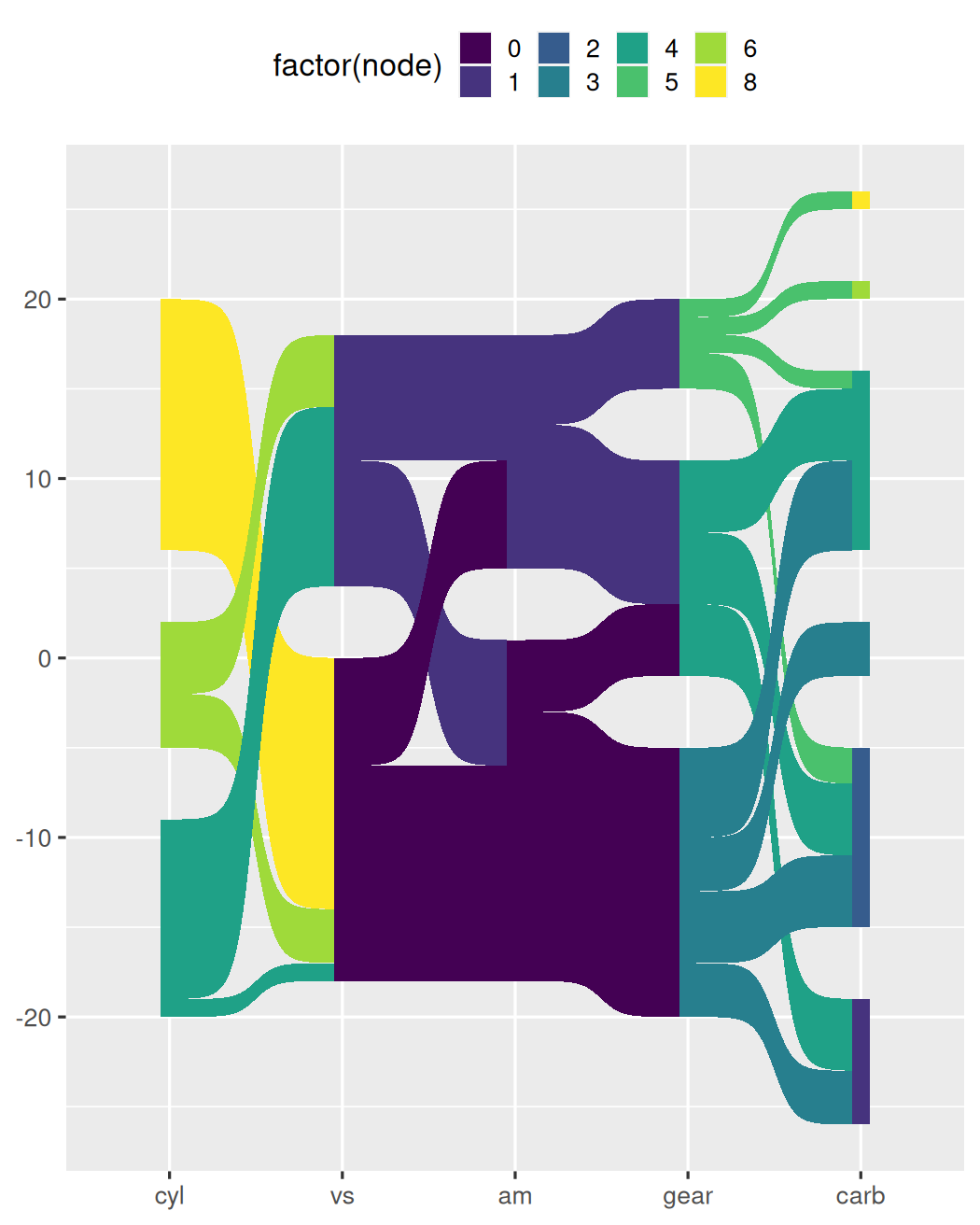
Flow Sankey / Alluvial
# remotes::install_github(# "davidsjoberg/ggsankey")df <- mtcars |> ggsankey::make_long( cyl, vs, am, gear, carb)ggplot(df) + aes(x, next_x=next_x, node=node, next_node=next_node, fill=factor(node)) + ggsankey::geom_sankey( flow.alpha=0.6, node.color="gray30") + scale_fill_viridis_d() + labs(x=NULL) + theme(legend.position="top")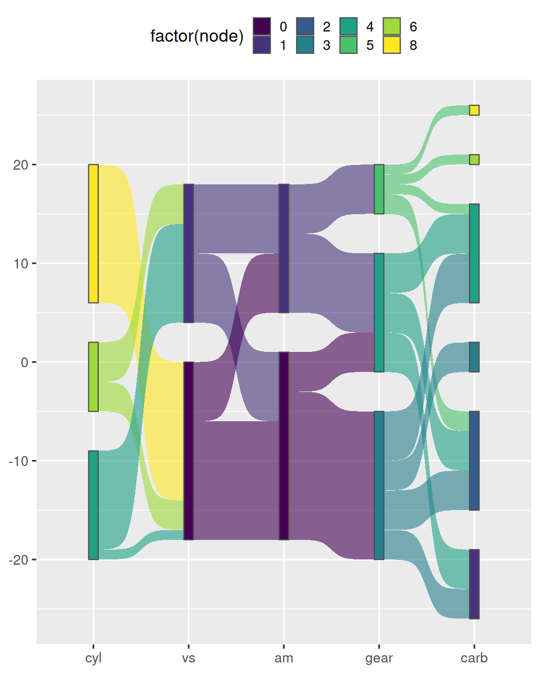
Flow Sankey / Alluvial
# remotes::install_github(# "davidsjoberg/ggsankey")df <- mtcars |> ggsankey::make_long( cyl, vs, am, gear, carb)ggplot(df) + aes(x, next_x=next_x, node=node, next_node=next_node, fill=factor(node), label=node) + ggsankey::geom_sankey( flow.alpha=0.6, node.color="gray30") + ggsankey::geom_sankey_label( size=3, color="white", fill="gray40") + scale_fill_viridis_d() + labs(x=NULL) + theme(legend.position="none")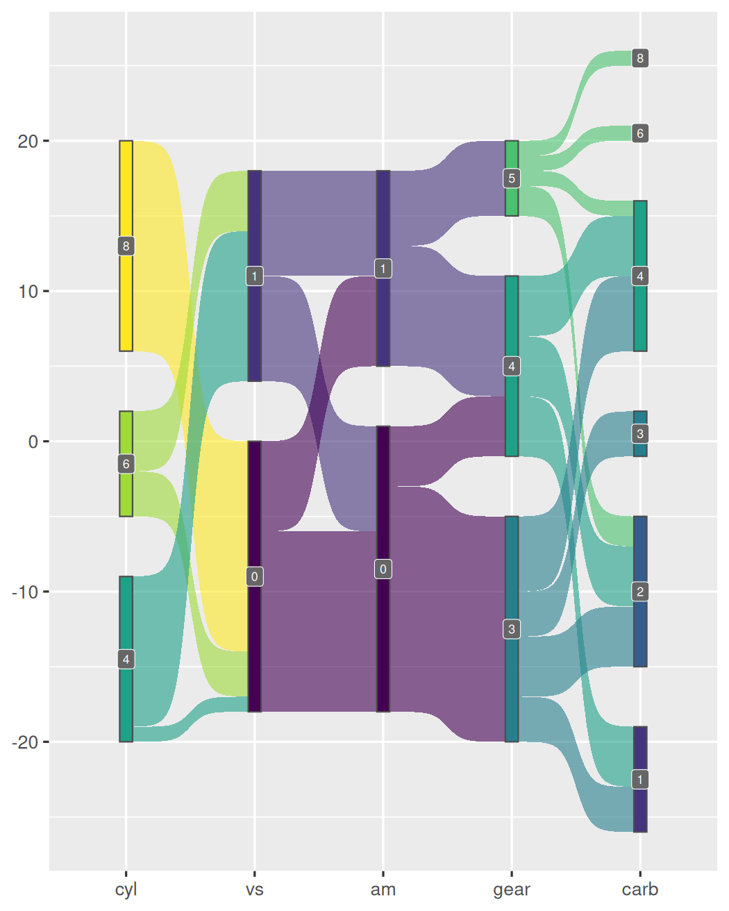
Flow Sankey / Alluvial
# remotes::install_github(# "davidsjoberg/ggsankey")df <- mtcars |> ggsankey::make_long( cyl, vs, am, gear, carb)ggplot(df) + aes(x, next_x=next_x, node=node, next_node=next_node, fill=factor(node), label=node) + ggsankey::geom_sankey( flow.alpha=0.6, node.color="gray30") + ggsankey::geom_sankey_label( size=3, color="white", fill="gray40") + scale_fill_viridis_d() + ggsankey::theme_sankey(base_size=16) + labs(x=NULL) + theme(legend.position="none")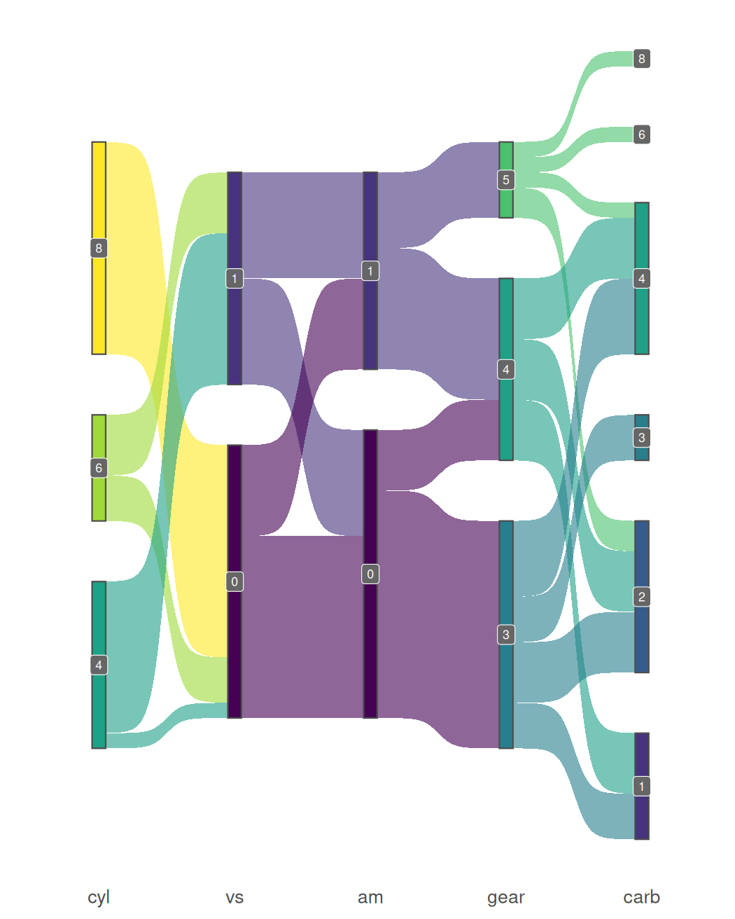
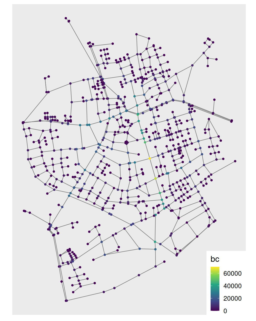
Flow  Geospatial network
library(tidygraph)library(sfnetworks)net <- as_sfnetwork(roxel, directed=F) |> activate("nodes") |> mutate(bc = centrality_betweenness())ggplot() + geom_sf(data=sf::st_as_sf(net, "edges"), color="grey50") + geom_sf(data=sf::st_as_sf(net, "nodes"), aes(color=bc)) + scale_color_viridis_c() + theme(legend.position=c(1, 0), legend.justification=c(1, 0))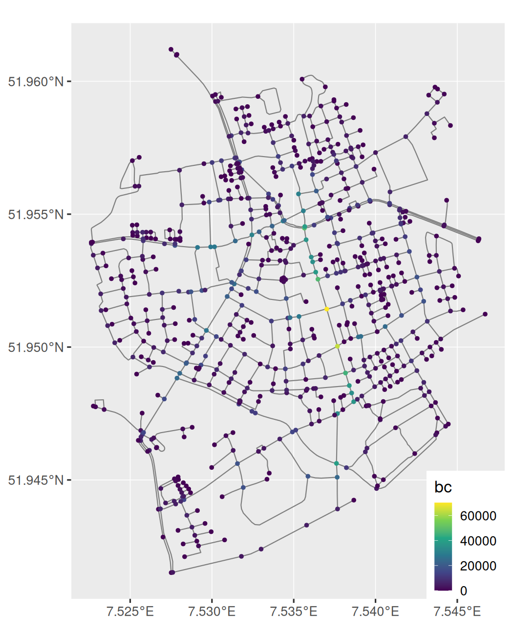
Flow Geospatial network
library(ggraph)library(tidygraph)library(sfnetworks)net <- as_sfnetwork(roxel, directed=F) |> activate("nodes") |> mutate(bc = centrality_betweenness())ggraph(net) + geom_edge_link(color="grey50") + geom_node_point(aes(color=bc)) + scale_color_viridis_c() + theme(legend.position=c(1, 0), legend.justification=c(1, 0))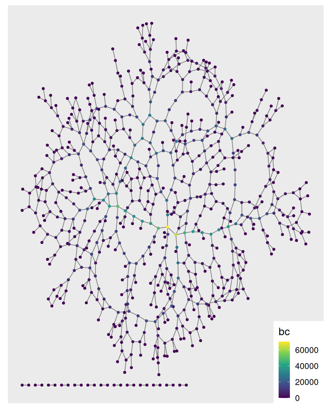
Flow Geospatial network
library(ggraph)library(tidygraph)library(sfnetworks)net <- as_sfnetwork(roxel, directed=F) |> activate("nodes") |> mutate(bc = centrality_betweenness())layout_sf <- function(graph) { graph <- activate(graph, "nodes") data.frame( x=sf::st_coordinates(graph)[,"X"], y=sf::st_coordinates(graph)[,"Y"])} ggraph(net, layout=layout_sf) + geom_edge_link(color="grey50") + geom_node_point(aes(color=bc)) + scale_color_viridis_c() + theme(legend.position=c(1, 0), legend.justification=c(1, 0))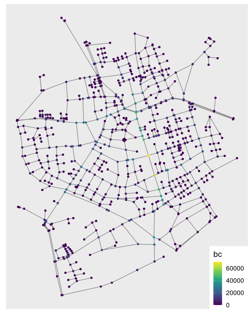
Flow Geospatial network
library(ggraph)library(tidygraph)library(sfnetworks)net <- as_sfnetwork(roxel, directed=F) |> activate("nodes") |> mutate(bc = centrality_betweenness())layout_sf <- function(graph) { graph <- activate(graph, "nodes") data.frame( x=sf::st_coordinates(graph)[,"X"], y=sf::st_coordinates(graph)[,"Y"])}ggraph(net, layout=layout_sf) + geom_edge_link(color="grey50") + geom_node_point(aes(color=bc)) + coord_sf(crs=sf::st_crs(net)) + scale_color_viridis_c() + theme(legend.position=c(1, 0), legend.justification=c(1, 0))