Directory of Visualizations
Based on The R Graph Gallery


Part of a Whole


Grouped and Stacked barplot Treemap Doughnut Pie chart Dendrogram Circular packing
- Visualization of proportions
- Some charts are also able to convey hierarchies
- Some are rarely appropriate
Part of a Whole Stacked barplot
mpg |> count(drv, class, name="count") |>ggplot() + aes(count, reorder(class, count, sum)) + geom_col(aes(fill=drv)) + labs(y=NULL) + theme(legend.position="top")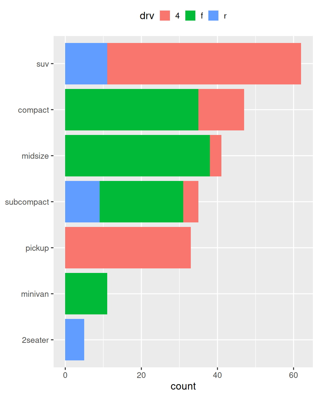
Part of a Whole Stacked barplot
mpg |> count(drv, class, name="count") |> group_by(class) |> mutate(prop = count / sum(count)) |>ggplot() + aes(prop, reorder(class, count, sum)) + geom_col(aes(fill=drv)) + labs(y=NULL) + theme(legend.position="top")
Part of a Whole Stacked barplot
mpg |> count(drv, class, name="count") |> group_by(class) |> mutate(prop = count / sum(count)) |>ggplot() + aes(prop, reorder(class, count, sum)) + geom_col(aes(fill=drv)) + scale_x_continuous( label=scales::percent) + labs(y=NULL) + theme(legend.position="top")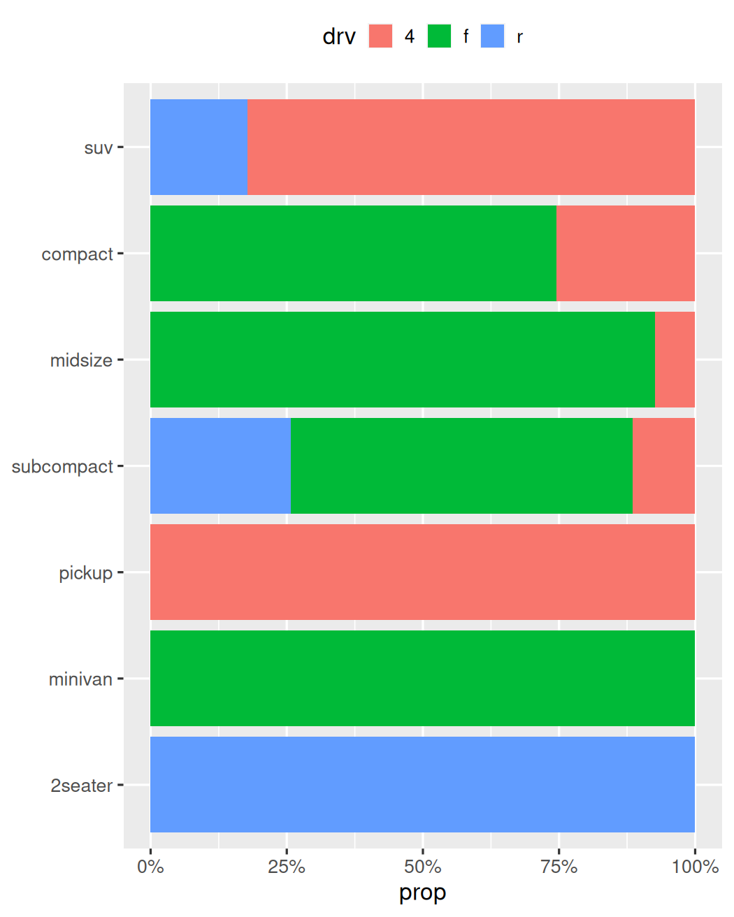
Part of a Whole Pie chart
data.frame( category=c("A", "B", "C"), prop=c(0.1, 0.6, 0.3)) |>ggplot() + aes(1, prop) + geom_col(aes(fill=category))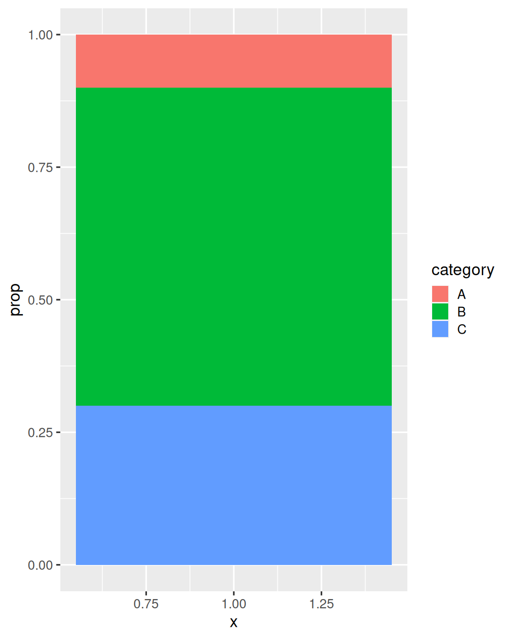
Part of a Whole Pie chart
data.frame( category=c("A", "B", "C"), prop=c(0.1, 0.6, 0.3)) |>ggplot() + aes(1, prop) + geom_col(aes(fill=category)) + coord_polar(theta="y") + theme_void(base_size=16)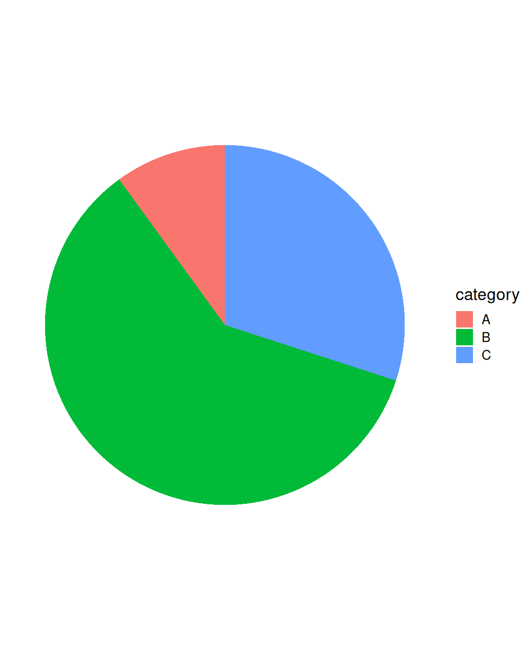
Part of a Whole Doughnut
data.frame( category=c("A", "B", "C"), prop=c(0.1, 0.6, 0.3)) |>ggplot() + aes(1, prop) + geom_col(aes(fill=category)) + xlim(c(-0.5, 1.5))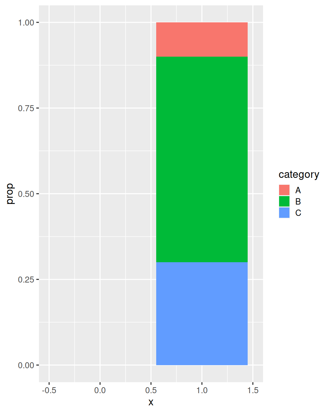
Part of a Whole Doughnut
data.frame( category=c("A", "B", "C"), prop=c(0.1, 0.6, 0.3)) |>ggplot() + aes(1, prop) + geom_col(aes(fill=category)) + xlim(c(-0.5, 1.5)) + coord_polar(theta="y") + theme_void(base_size=16)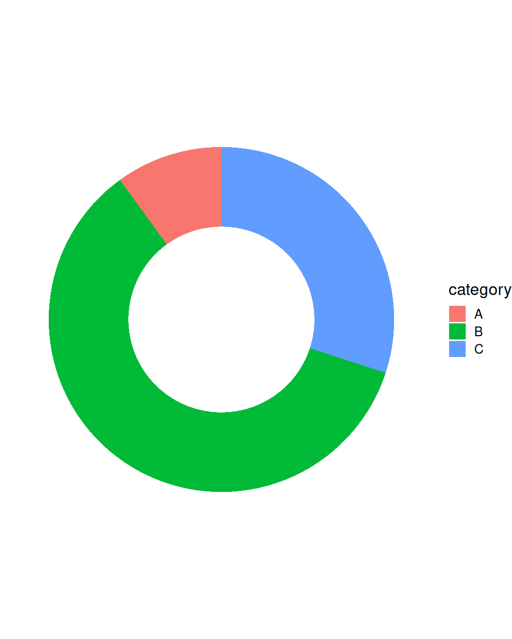
Part of a Whole Circular packing
library(packcircles)df <- mpg |> count(class, name="count")df <- cbind(df, circleProgressiveLayout( df$count, sizetype="area"))ggplot(df) + aes(x0=x, y0=y, r=radius) + ggforce::geom_circle()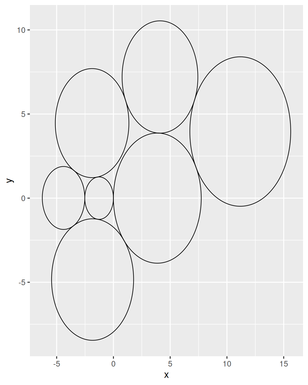
Part of a Whole Circular packing
library(packcircles)df <- mpg |> count(class, name="count")df <- cbind(df, circleProgressiveLayout( df$count, sizetype="area"))ggplot(df) + aes(x0=x, y0=y, r=radius) + ggforce::geom_circle(aes( fill=class), color=NA) + coord_fixed() + geom_text(aes(x, y, label=class)) + theme_void(base_size=16) + theme(legend.position="none")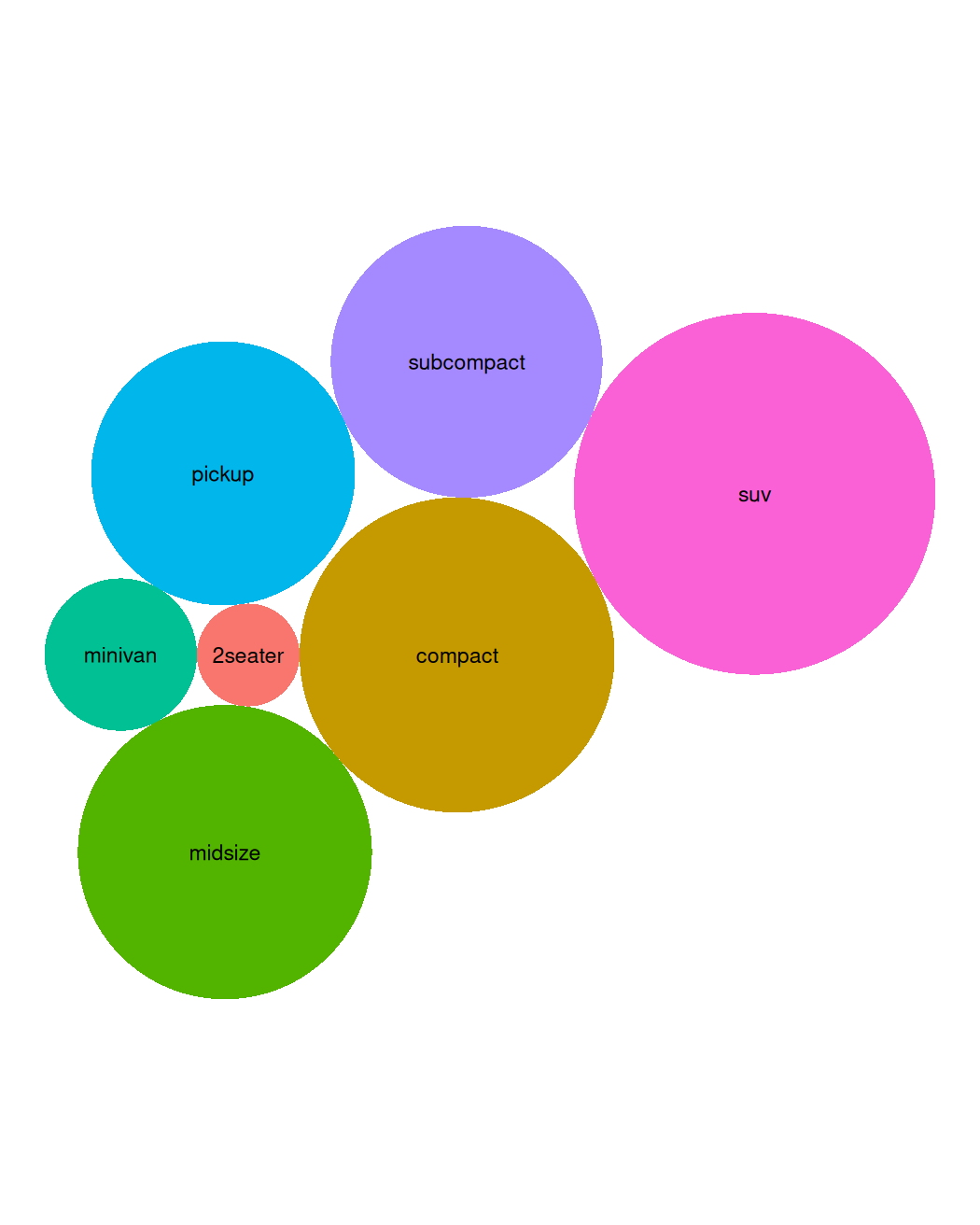
Part of a Whole Circular packing
library(packcircles)df <- data.frame( x = c(0, 1, 0, 1), y = c(0, 0, 1, 1), radius = c(0.7, 0.5, 0.6, 1.2))ggplot(df) + aes(x0=x, y0=y, r=radius) + ggforce::geom_circle() + geom_point(aes(x, y), color="red") + coord_fixed() + theme_void(base_size=16) + theme(legend.position="none")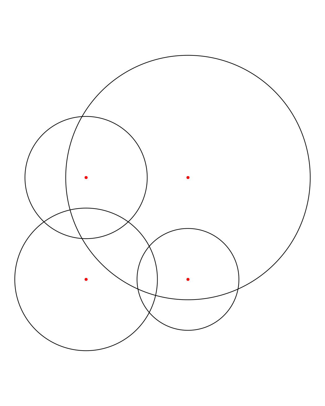
Part of a Whole Circular packing
library(packcircles)df <- data.frame( x = c(0, 1, 0, 1), y = c(0, 0, 1, 1), radius = c(0.7, 0.5, 0.6, 1.2))df.new <- circleRepelLayout( df, sizetype="radius")$layoutggplot(df.new) + aes(x0=x, y0=y, r=radius) + ggforce::geom_circle() + geom_point(aes(x, y), color="red") + geom_point(aes(x, y), df) + coord_fixed() + theme_void(base_size=16) + theme(legend.position="none")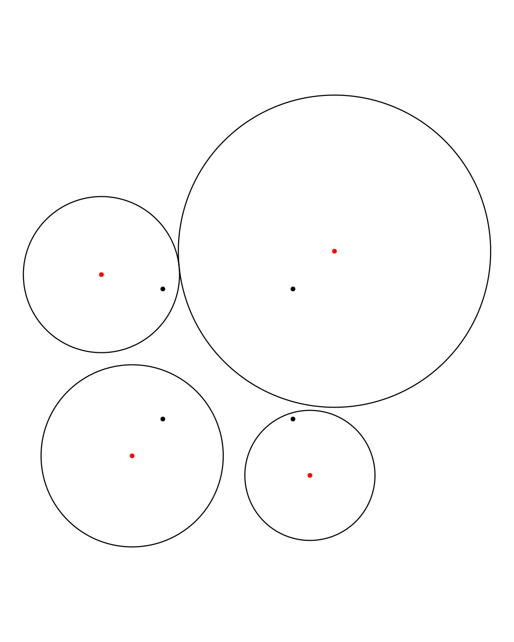
Part of a Whole Circular packing
edges <- ggraph::flare$edgesvertices <- ggraph::flare$verticesgraph <- igraph::graph_from_data_frame( edges, vertices=vertices)ggraph::ggraph(graph, layout="circlepack", weight=size) + ggraph::geom_node_circle() + theme_void(base_size=16)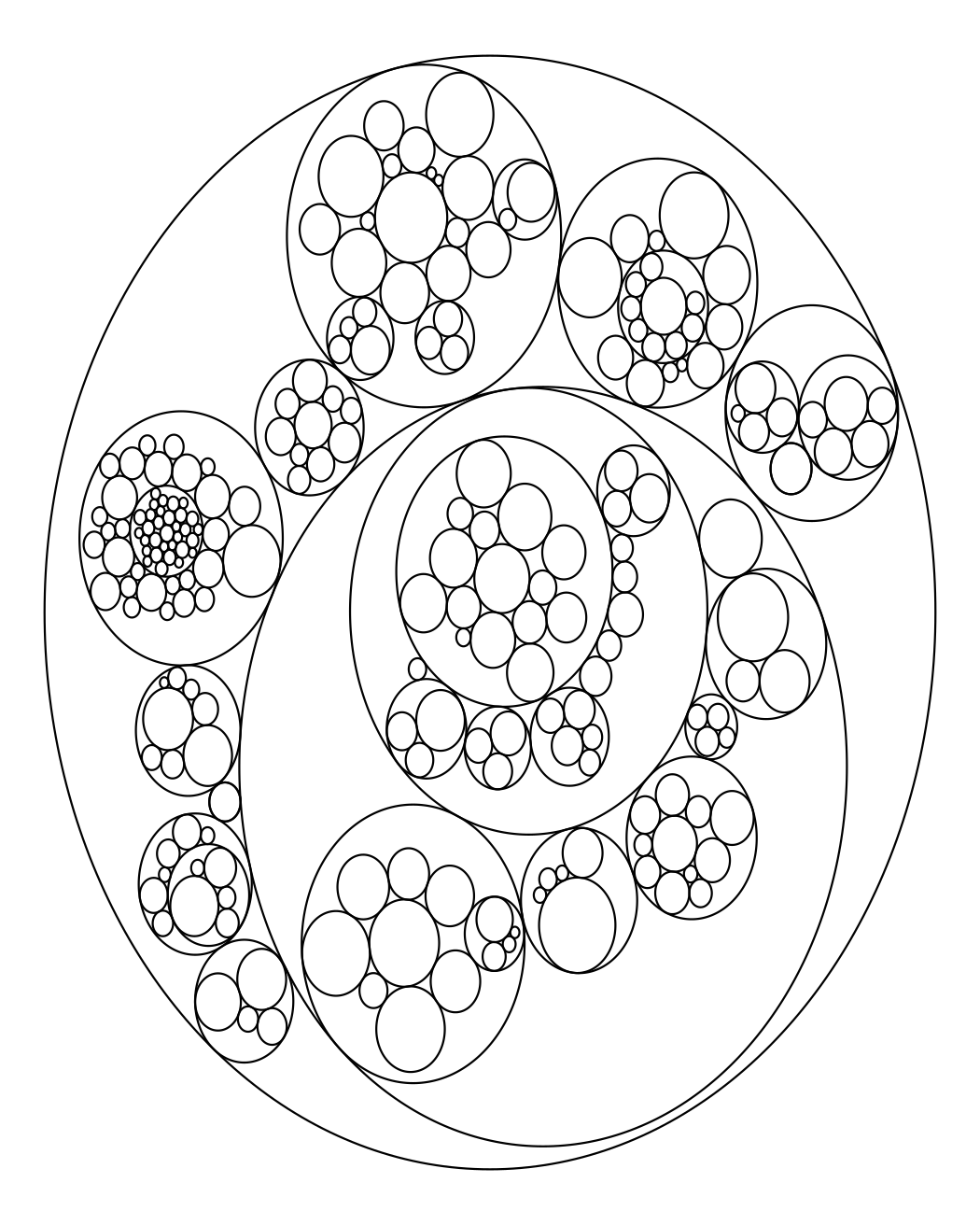
Part of a Whole Circular packing
edges <- ggraph::flare$edgesvertices <- ggraph::flare$verticesgraph <- igraph::graph_from_data_frame( edges, vertices=vertices)ggraph::ggraph(graph, layout="circlepack", weight=size) + ggraph::geom_node_circle( aes(fill=depth)) + scale_fill_viridis_c() + coord_fixed() + theme_void(base_size=16)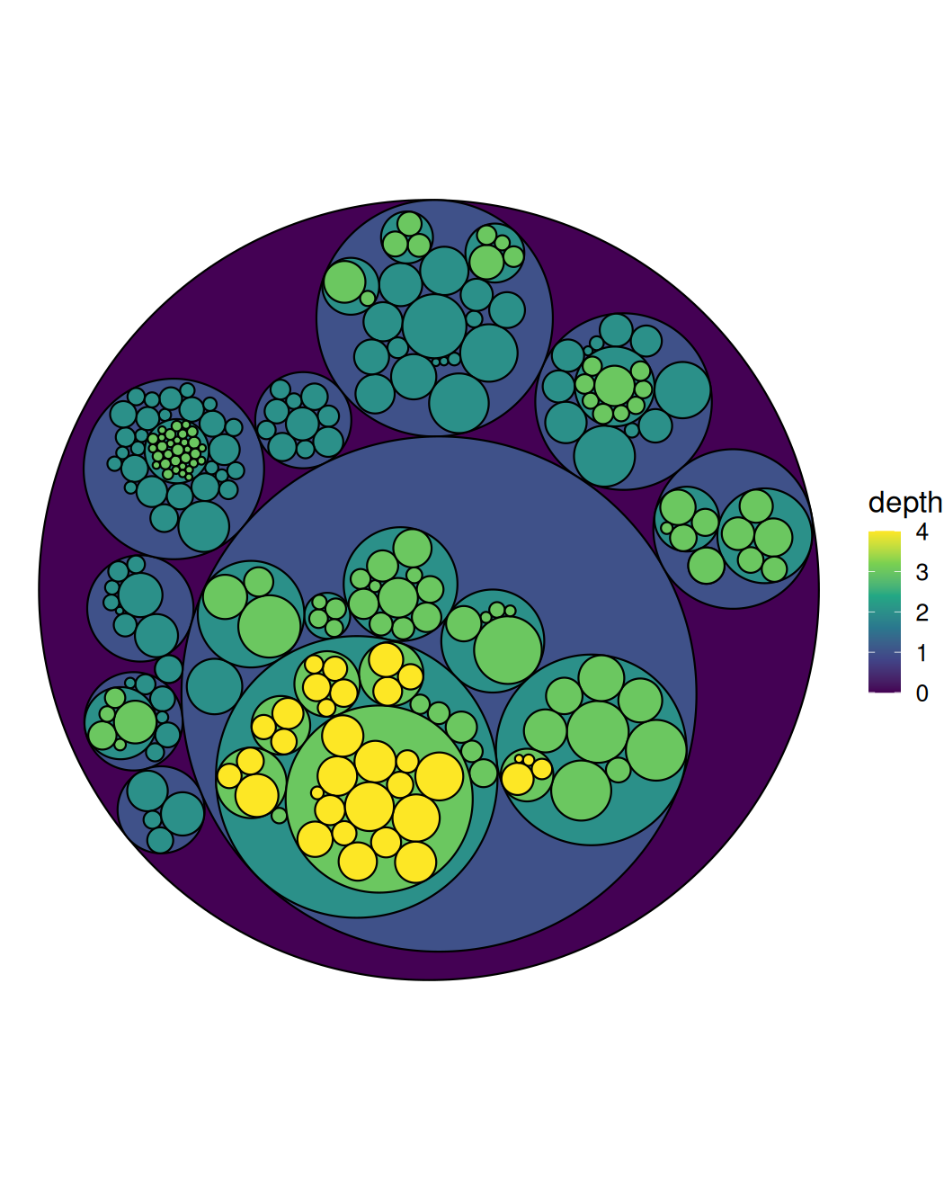
Part of a Whole Treemap
edges <- ggraph::flare$edgesvertices <- ggraph::flare$verticesgraph <- igraph::graph_from_data_frame( edges, vertices=vertices)ggraph::ggraph(graph, layout="treemap", weight=size) + ggraph::geom_node_tile( aes(fill=depth)) + scale_fill_viridis_c() + theme_void(base_size=16)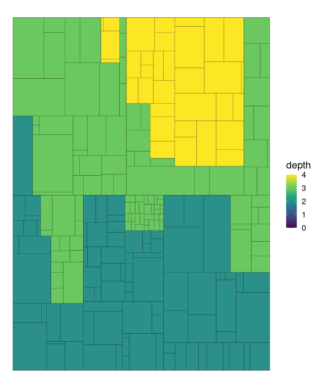
Part of a Whole Dendrogram
edges <- ggraph::flare$edgesvertices <- ggraph::flare$verticesgraph <- igraph::graph_from_data_frame( edges, vertices=vertices)ggraph::ggraph(graph, layout="tree") + ggraph::geom_edge_diagonal() + theme_void(base_size=16)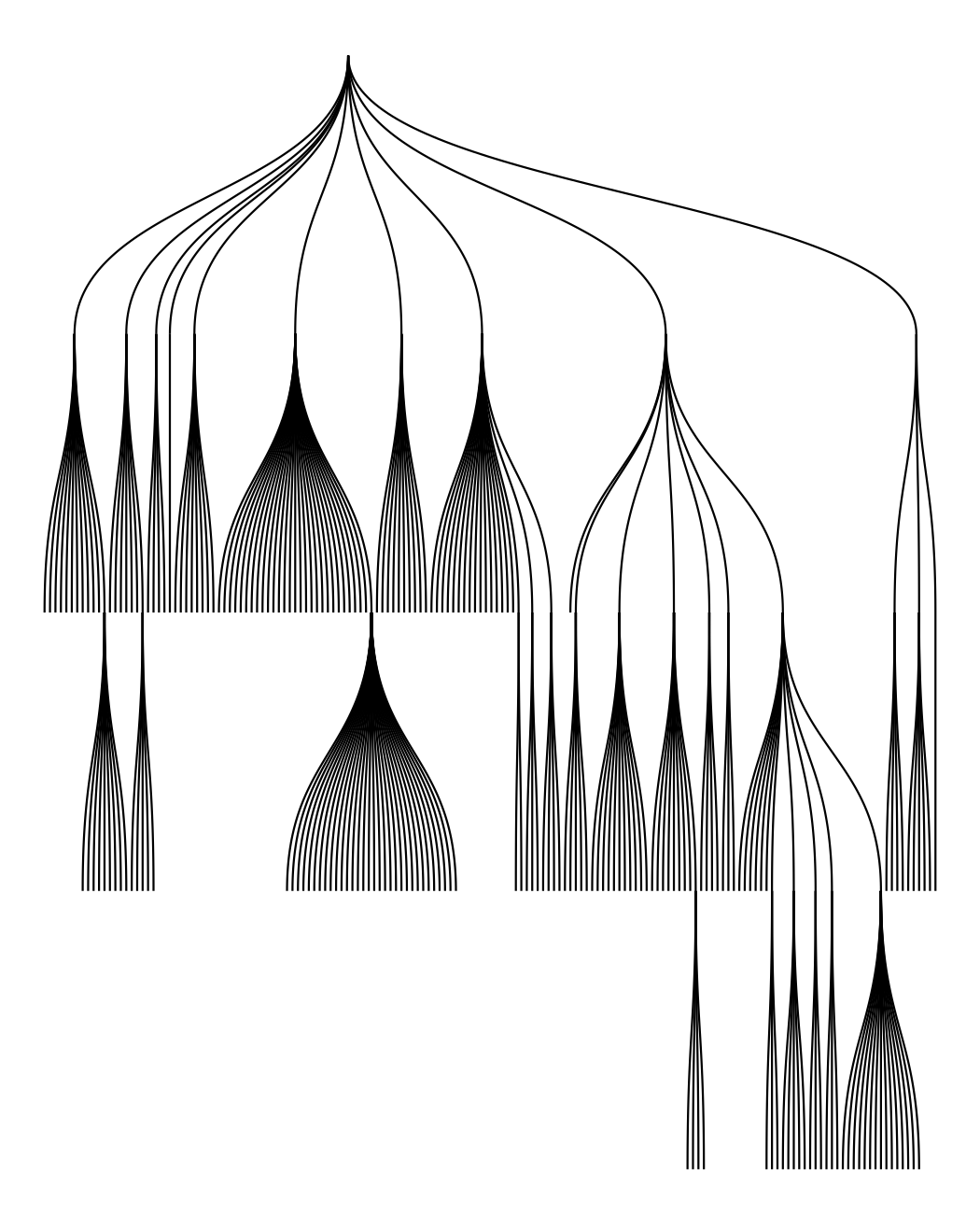
Part of a Whole Dendrogram
edges <- ggraph::flare$edgesvertices <- ggraph::flare$verticesgraph <- igraph::graph_from_data_frame( edges, vertices=vertices)ggraph::ggraph(graph, layout="dendrogram") + ggraph::geom_edge_diagonal() + theme_void(base_size=16)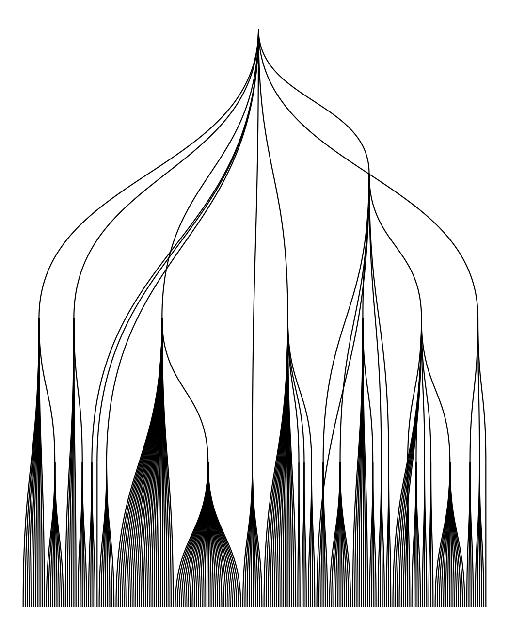
Part of a Whole Dendrogram
df <- hclust(dist(iris[, 1:4]))ggraph::ggraph(df, layout="dendrogram", height=height) + ggraph::geom_edge_elbow() + theme_void(base_size=16)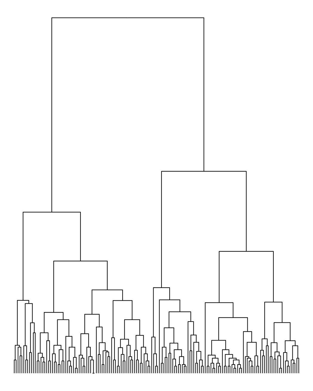
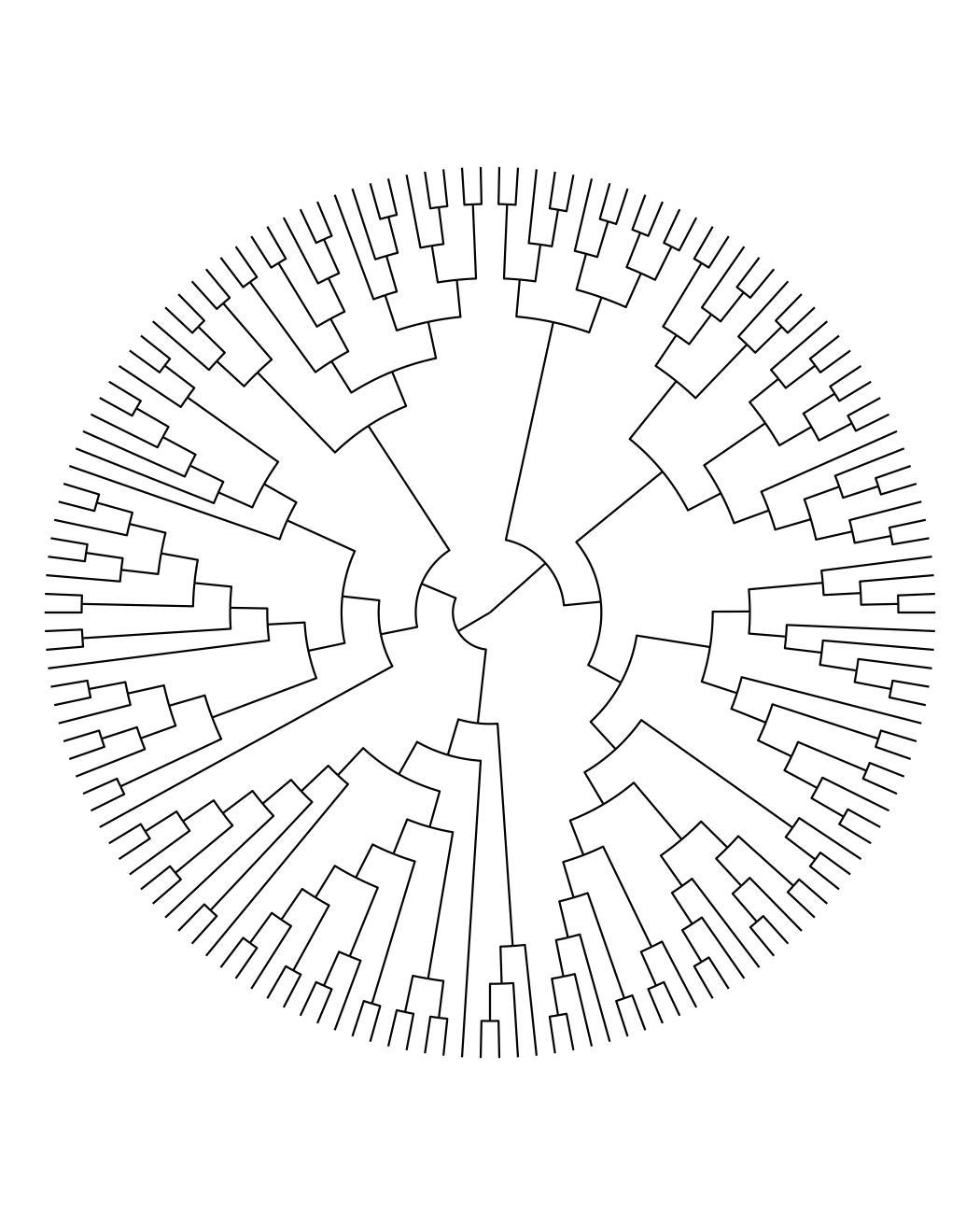
Part of a Whole Dendrogram
df <- hclust(dist(iris[, 1:4]))ggraph::ggraph(df, layout="dendrogram", circular=TRUE) + ggraph::geom_edge_elbow() + coord_fixed() + theme_void(base_size=16)