Directory of Visualizations
Based on The R Graph Gallery


Correlation


Scatter Heatmap Correlogram Bubble Connected scatter Density 2D
- Visualization of the relationship between two variables
- Two continuous, or two discrete, or mixed
- Options to include a third one
Correlation Scatter
gapminder::gapminder |> filter(year == 1997) |>ggplot() + aes(gdpPercap, lifeExp) + scale_x_log10() + geom_point()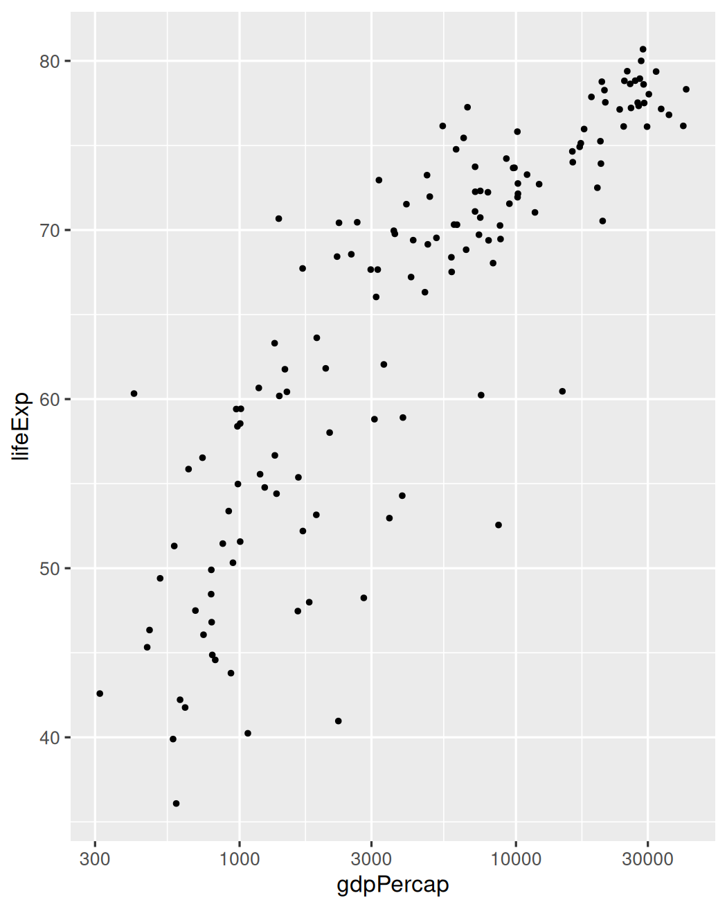
Correlation Scatter
gapminder::gapminder |> filter(year == 1997) |>ggplot() + aes(gdpPercap, lifeExp) + scale_x_log10() + geom_point(aes(color=continent)) + theme(legend.position=c(1, 0), legend.justification=c(1, 0))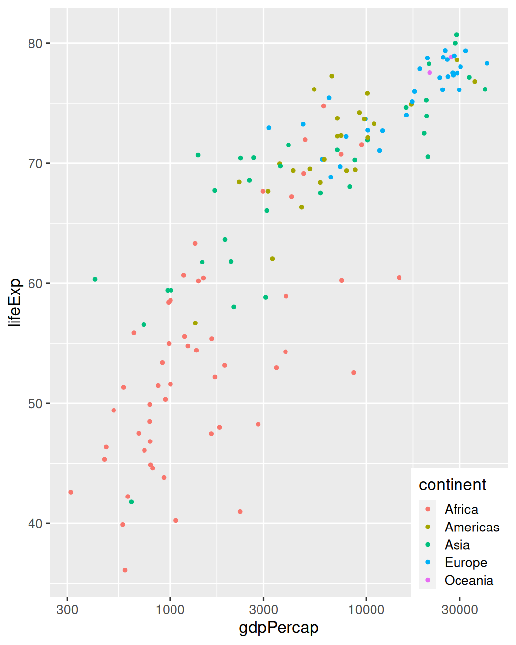
Correlation Bubble
gapminder::gapminder |> filter(year == 1997) |>ggplot() + aes(gdpPercap, lifeExp) + scale_x_log10() + geom_point(aes(color=continent, size=pop)) + theme(legend.position=c(1, 0), legend.justification=c(1, 0))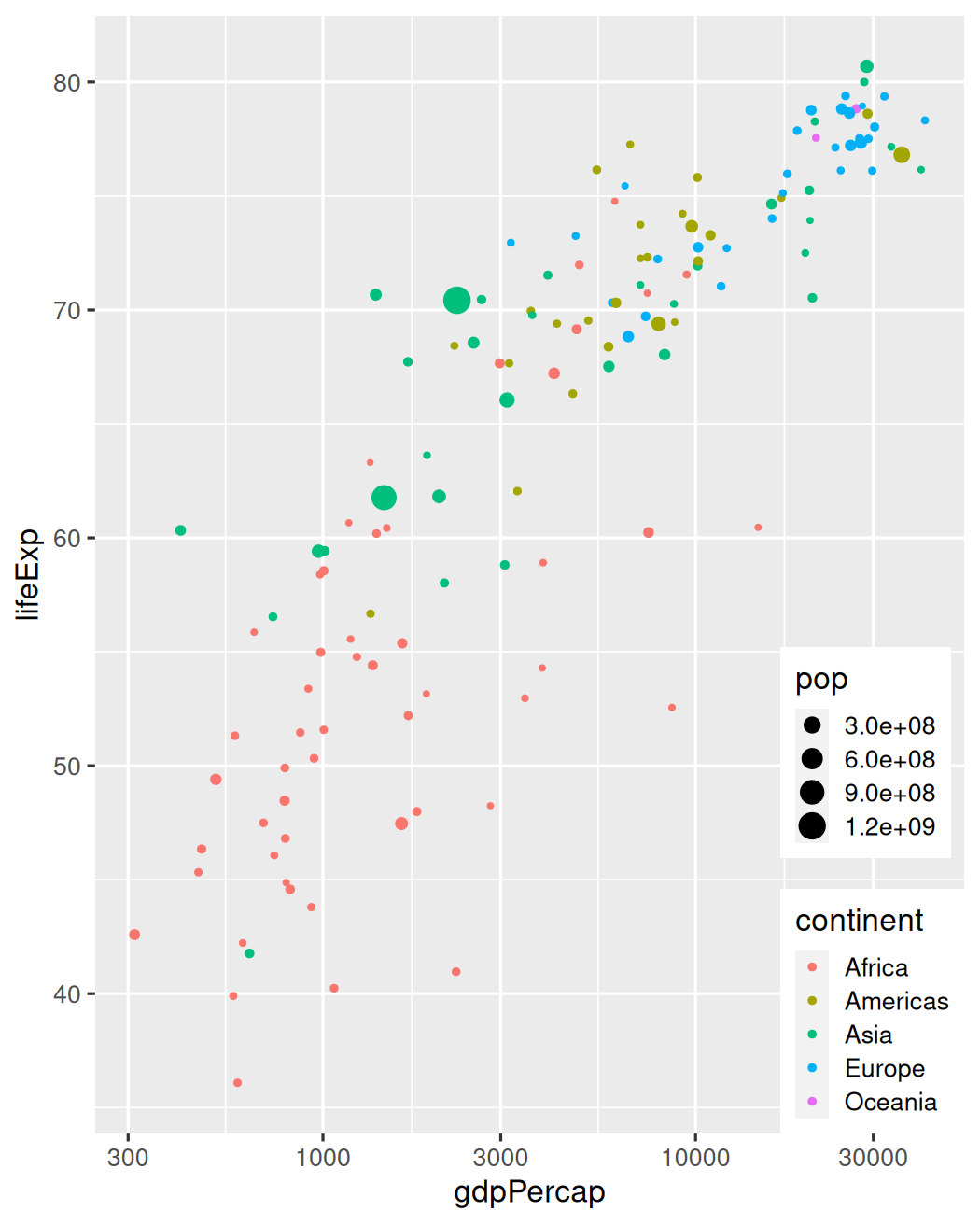
Correlation Bubble
gapminder::gapminder |> filter(year == 1997) |>ggplot() + aes(gdpPercap, lifeExp) + scale_x_log10() + geom_point(aes(color=continent, size=pop), alpha=0.7) + scale_size_area(max_size=20) + theme(legend.position=c(1, 0), legend.justification=c(1, 0))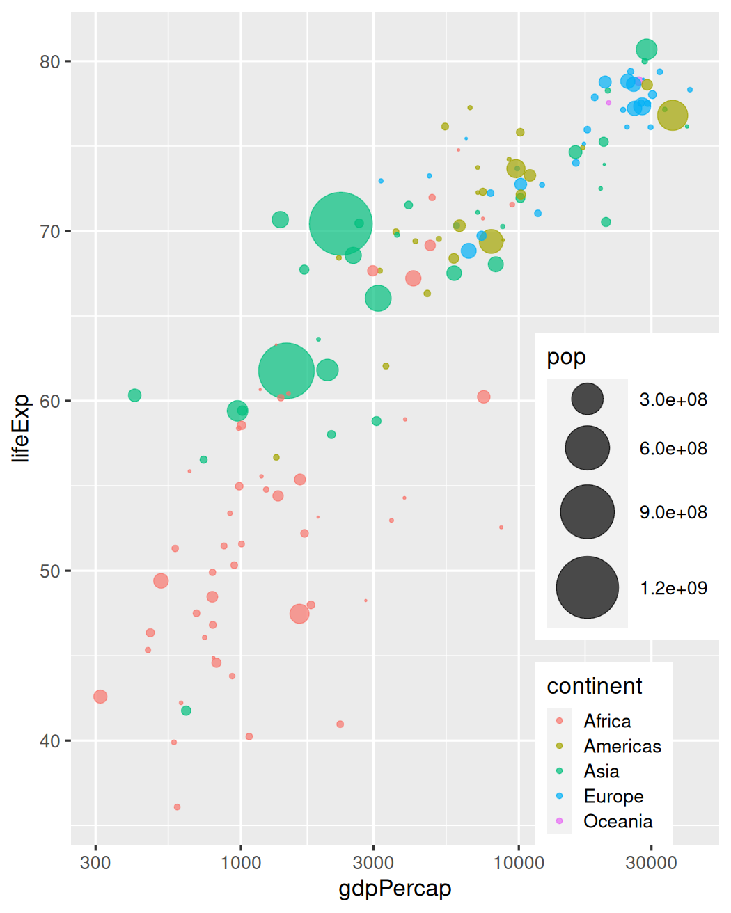
Correlation Bubble
gapminder::gapminder |> filter(year == 1997) |>ggplot() + aes(gdpPercap, lifeExp) + scale_x_log10() + geom_point(aes(color=continent, size=pop), alpha=0.7) + scale_size_area(max_size=20) + geom_smooth() + theme(legend.position=c(1, 0), legend.justification=c(1, 0))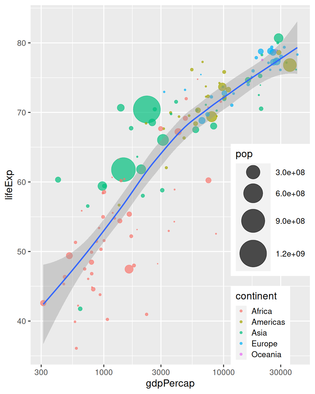
Correlation Bubble
gapminder::gapminder |> filter(year == 1997) |>ggplot() + aes(gdpPercap, lifeExp) + scale_x_log10() + geom_point(aes(color=continent, size=pop), alpha=0.7) + scale_size_area(max_size=20) + geom_smooth(method="lm") + theme(legend.position=c(1, 0), legend.justification=c(1, 0))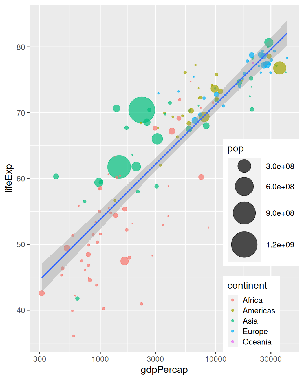
Correlation Connected Scatter
gapminder::gapminder |> filter(year == 1997) |>ggplot() + aes(gdpPercap, lifeExp) + scale_x_log10() + geom_point(aes(color=continent)) + geom_line(aes(color=continent)) + theme(legend.position=c(1, 0), legend.justification=c(1, 0))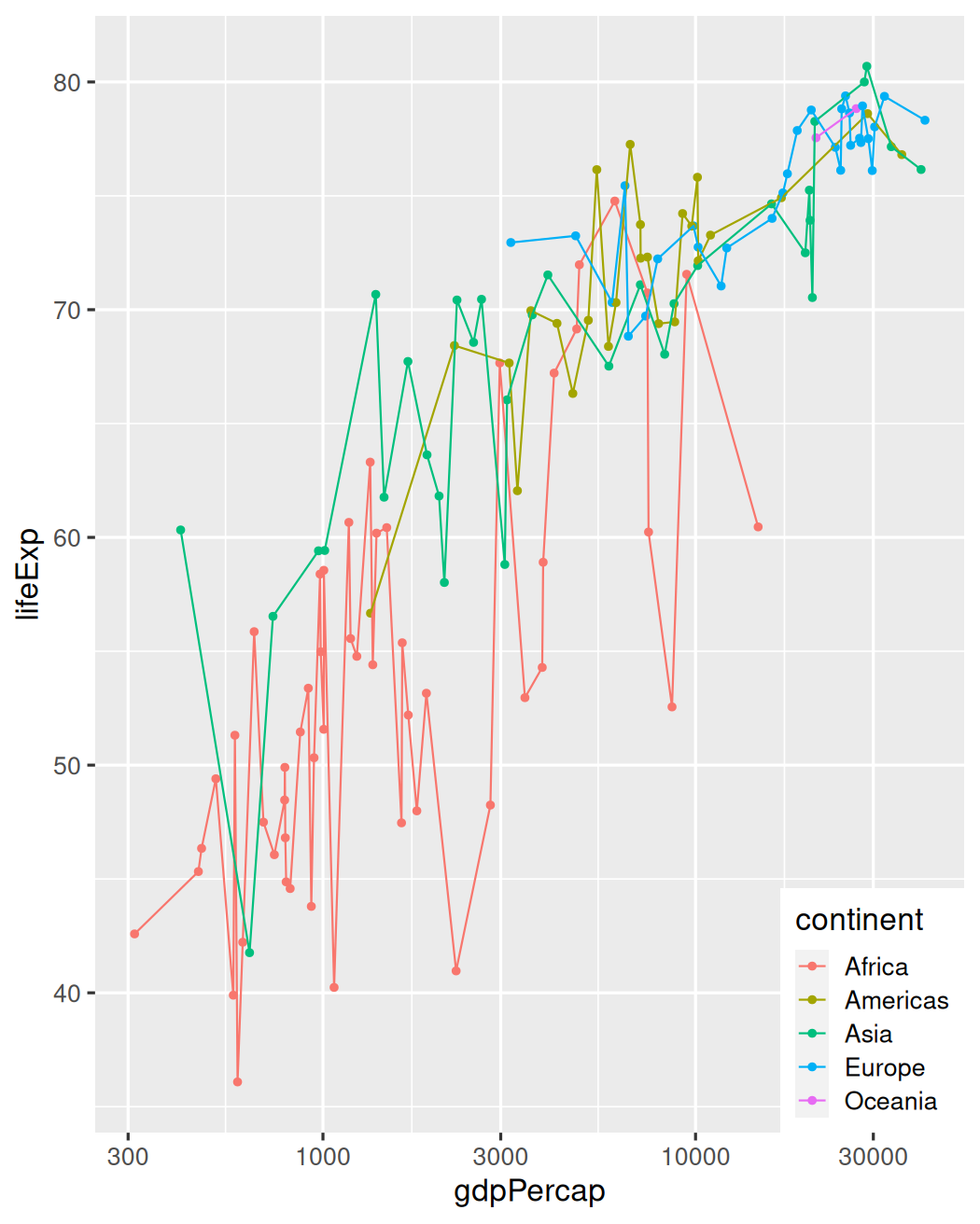
Correlation Connected Scatter
babynames::babynames |> filter(name %in% c( "Ashley", "Amanda")) |> filter(sex == "F") |> filter(year > 1970) |> select(year, name, n) |> spread(key = name, value=n, -1) |>ggplot() + aes(Amanda, Ashley, color=year) + geom_point() + geom_path() + scale_color_viridis_c() + theme(legend.position=c(0, 1), legend.justification=c(0, 1))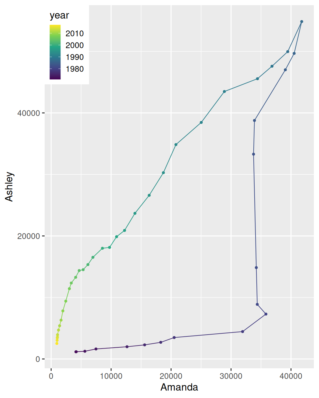
Correlation Connected Scatter
df <- babynames::babynames |> filter(name %in% c( "Ashley", "Amanda")) |> filter(sex == "F") |> filter(year > 1970) |> select(year, name, n) |> spread(key = name, value=n, -1)text <- df |> filter(year %in% c( 1972, 1980, 1984, 1987, 2012))ggplot(df) + aes(Amanda, Ashley, color=year) + geom_path(arrow=arrow( angle=15, type="closed", length=unit(0.1, "inches"))) + scale_color_viridis_c() + geom_label(aes(label=year), text) + theme(legend.position=c(0, 1), legend.justification=c(0, 1))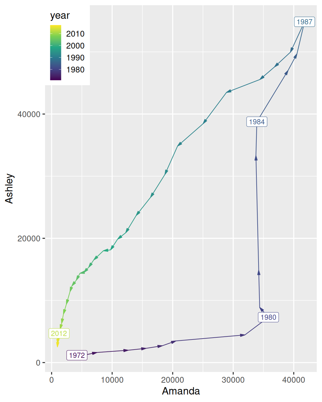
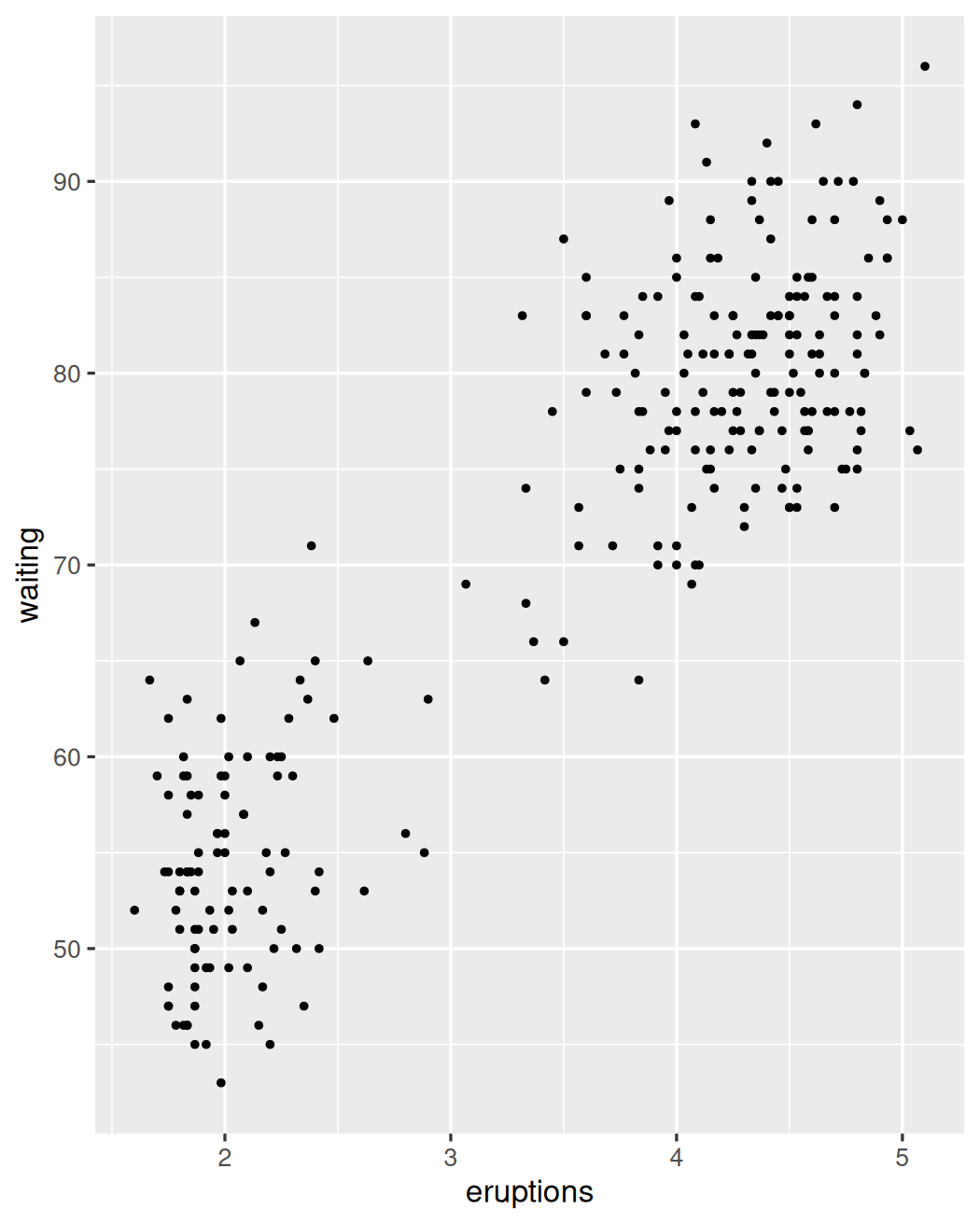
Correlation Scatter
ggplot(faithful) + aes(eruptions, waiting) + geom_point() + ggside::geom_xsidehistogram()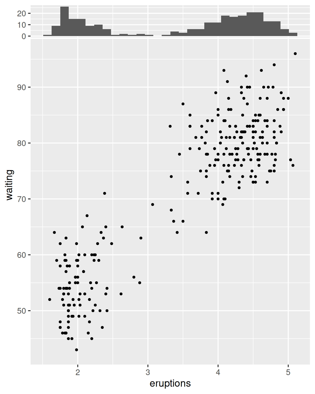
Correlation Density 2D
ggplot(faithful) + aes(eruptions, waiting) + geom_bin2d() + scale_fill_viridis_c() + ggside::geom_xsidehistogram() + theme(legend.position=c(1, 0), legend.justification=c(1, 0))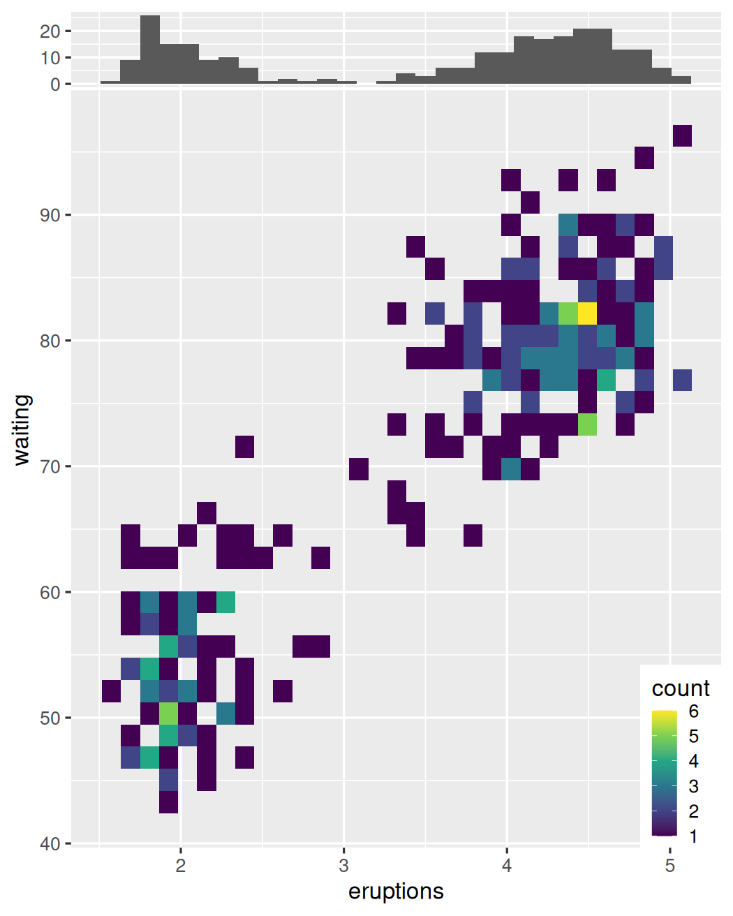
Correlation Density 2D
ggplot(faithful) + aes(eruptions, waiting) + geom_hex() + scale_fill_viridis_c() + ggside::geom_xsidehistogram() + theme(legend.position=c(1, 0), legend.justification=c(1, 0))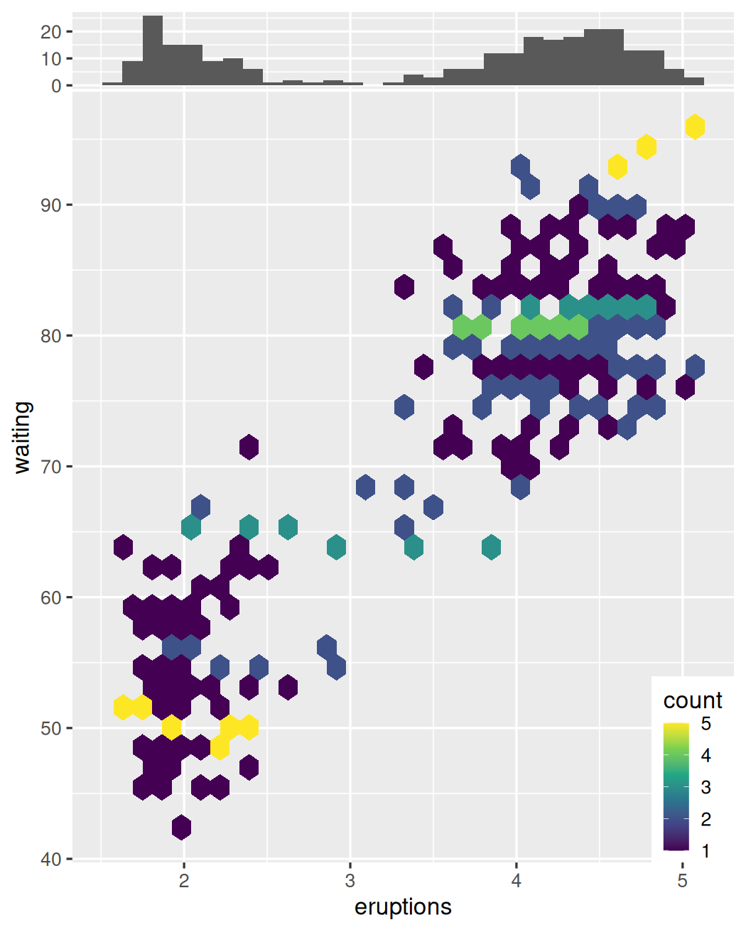
Correlation Density 2D
ggplot(faithful) + aes(eruptions, waiting) + geom_density2d_filled() + ggside::geom_xsidehistogram() + theme(legend.position=c(1, 0), legend.justification=c(1, 0))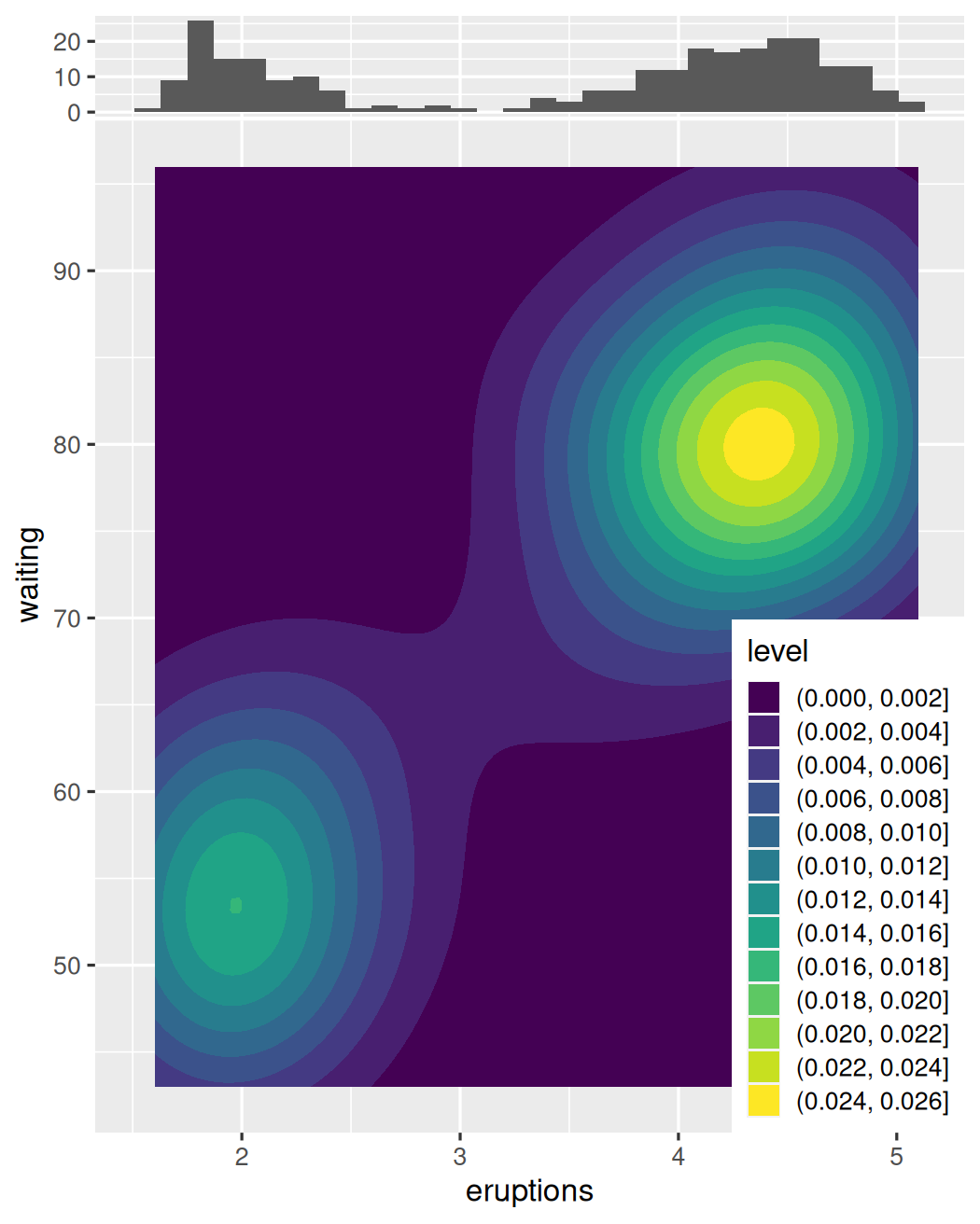
Correlation Density 2D
ggplot(faithfuld) + aes(eruptions, waiting, fill=density) + geom_raster() + scale_fill_viridis_c() + theme(legend.position=c(1, 0), legend.justification=c(1, 0))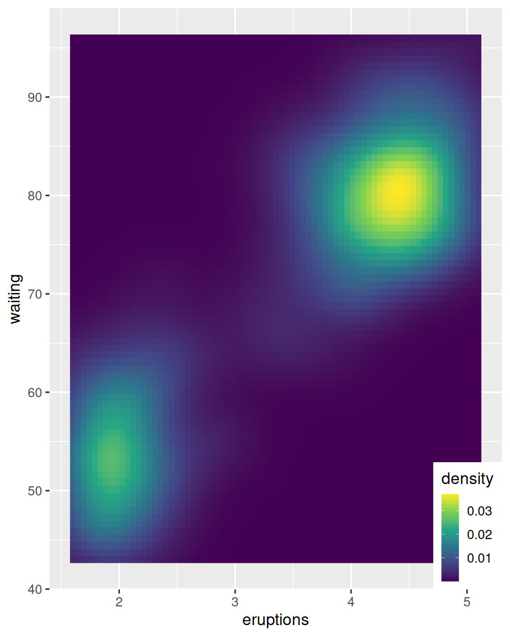
Correlation Density 2D
ggplot(faithfuld) + aes(eruptions, waiting, fill=density) + geom_raster(interpolate=TRUE) + scale_fill_viridis_c() + theme(legend.position=c(1, 0), legend.justification=c(1, 0))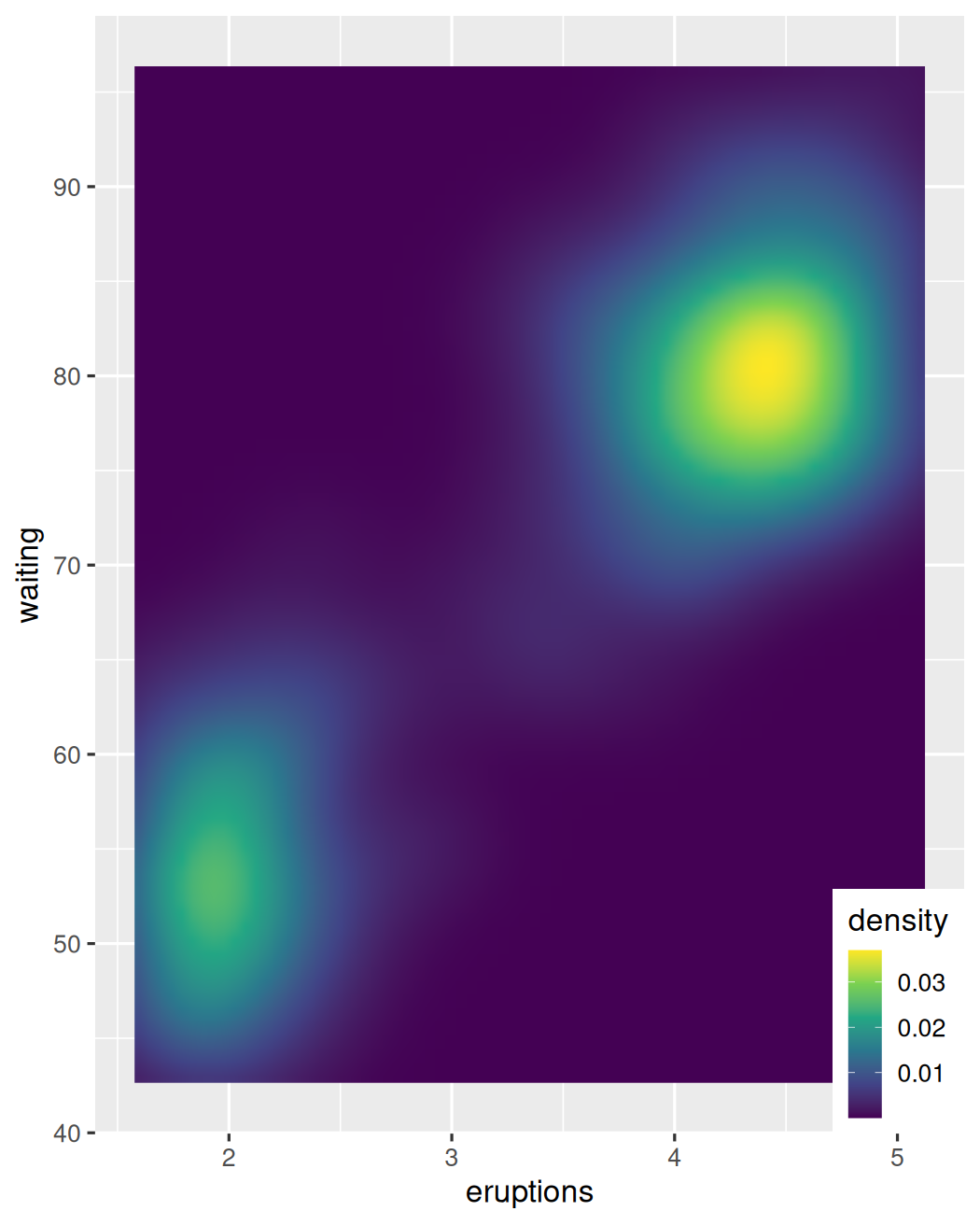
Correlation Heatmap
mtcars |> tibble::rownames_to_column("model") |> gather("key", "value", -model) |>ggplot() + aes(key, model, fill=value) + geom_tile() + scale_fill_viridis_c( trans="pseudo_log") + labs(x=NULL, y=NULL)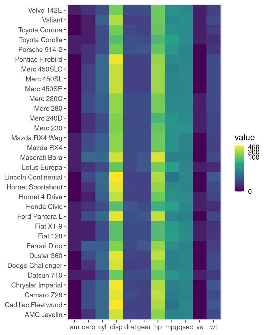
Correlation Correlogram
mtcars |> cor(mtcars) |> ggcorrplot::ggcorrplot() + theme(legend.position="top")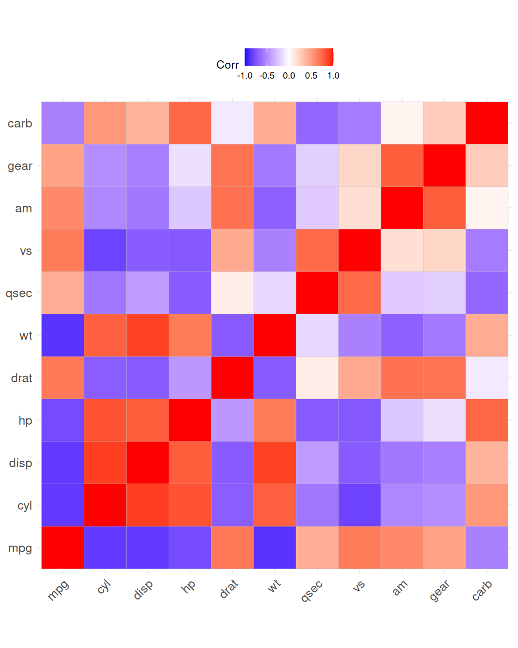
Correlation Correlogram
mtcars |> cor(mtcars) |> ggcorrplot::ggcorrplot( hc.order=TRUE, outline.color="white") + theme(legend.position="top")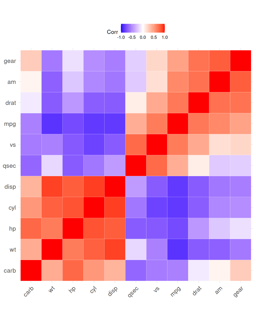
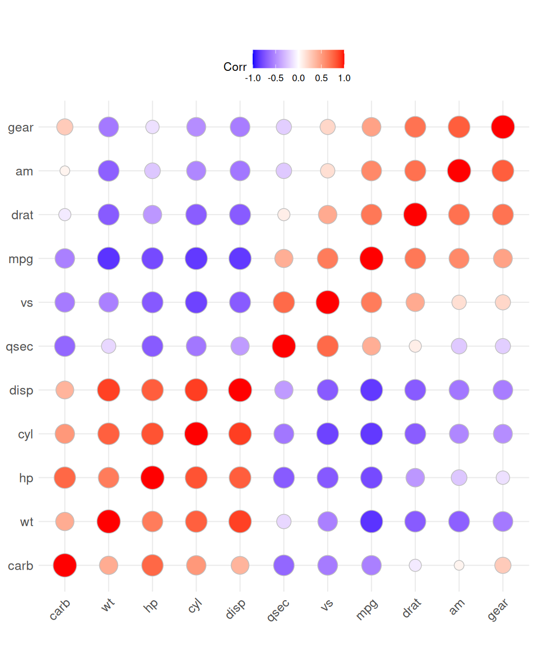
Correlation Correlogram
mtcars |> cor(mtcars) |> ggcorrplot::ggcorrplot( hc.order=TRUE, method="circle") + theme(legend.position="top")