Directory of Visualizations
Based on The R Graph Gallery


Distribution


Violin Density Histogram Boxplot Ridgeline
- Visualization of one or multiple univariate distributions
- Stacked versions are difficult to interpret and should be avoided
- Some require fine-tuning of the parameters to avoid being misleading
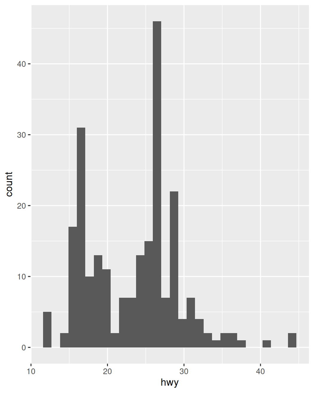

Distribution Histogram
ggplot(mpg) + aes(hwy, fill=class) + geom_histogram() + theme(legend.position=c(1, 1), legend.justification=c(1, 1))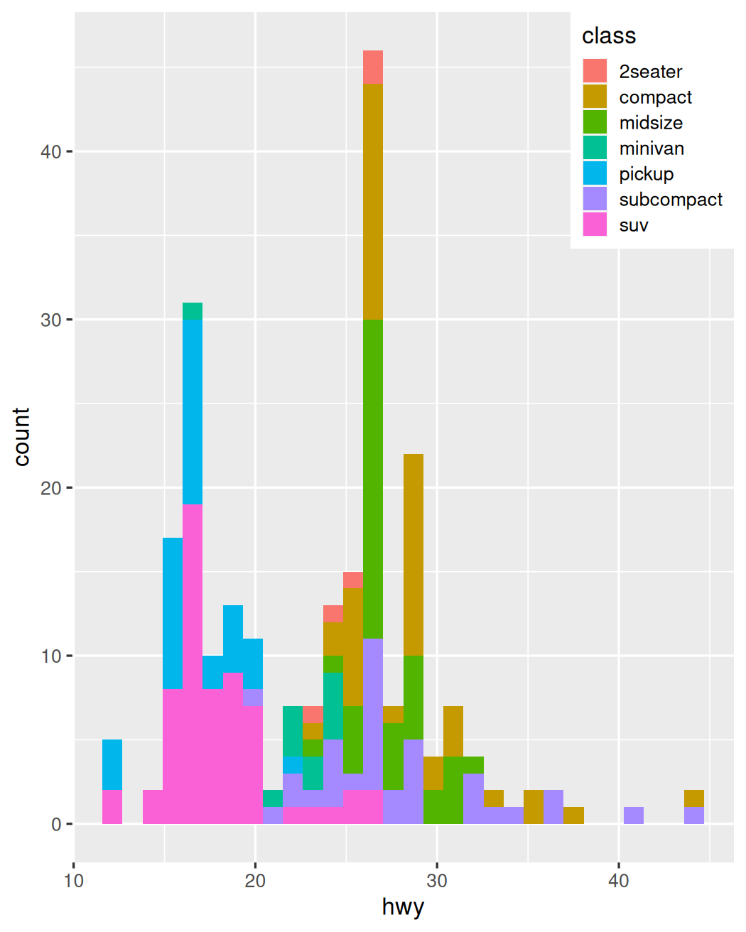
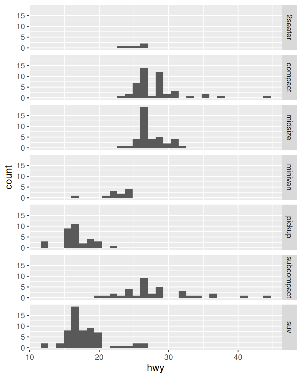
Distribution Histogram
ggplot(mpg) + aes(hwy) + geom_histogram() + facet_grid( reorder(class, -hwy, median) ~ .)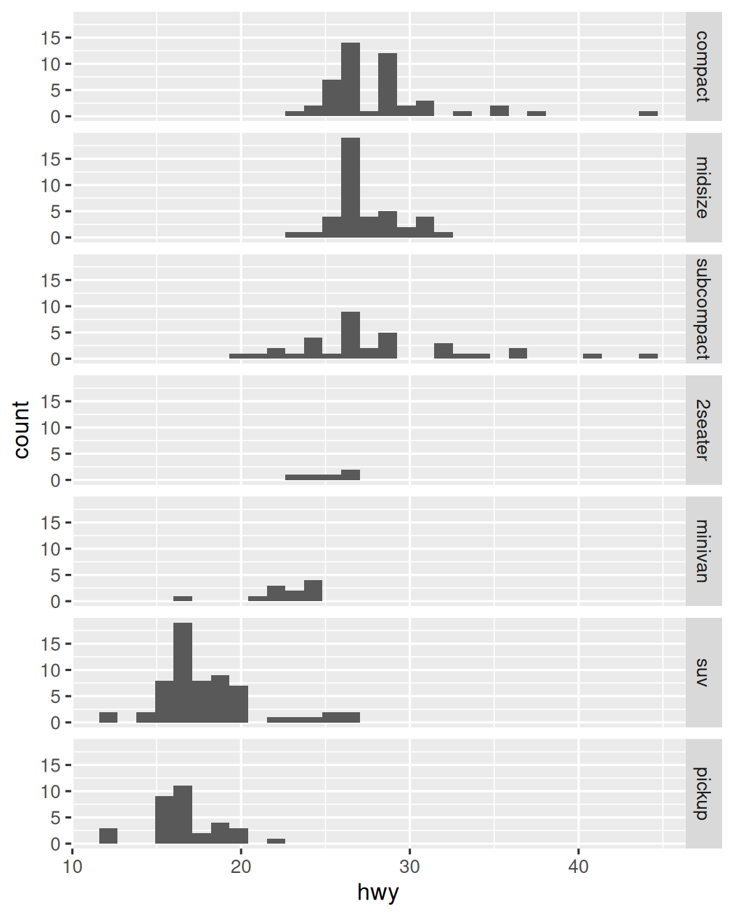
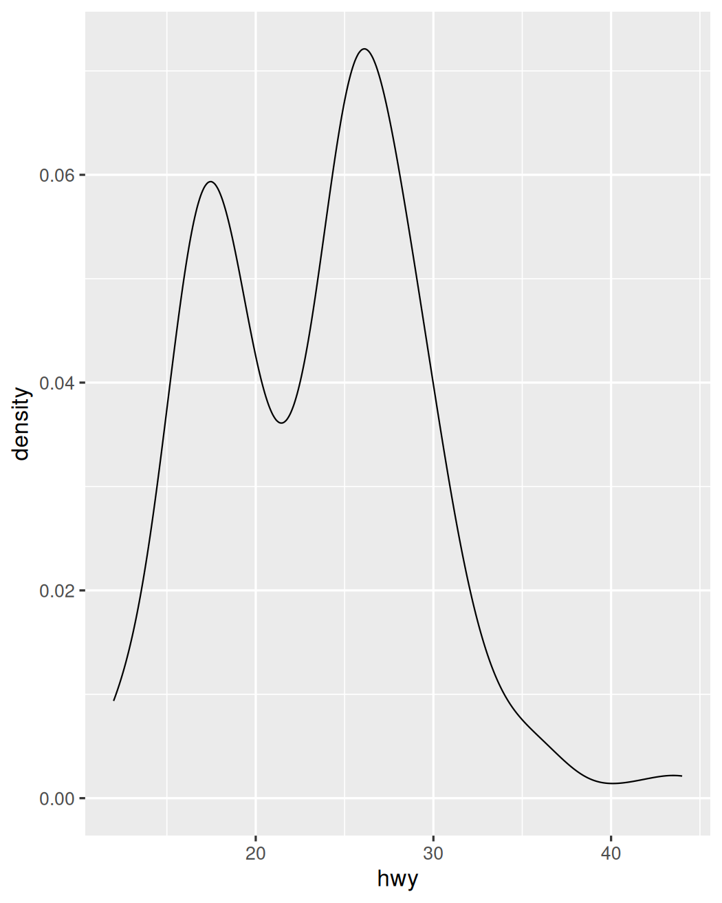
Distribution Density
ggplot(mpg) + aes(hwy, after_stat(density)) + geom_histogram(fill="gray") + geom_density()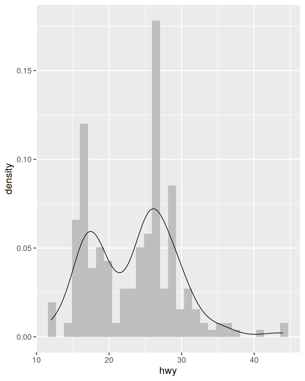
Distribution Density
ggplot(mpg) + aes(hwy, after_stat(density)) + geom_histogram(fill="gray") + geom_density(adjust=0.2)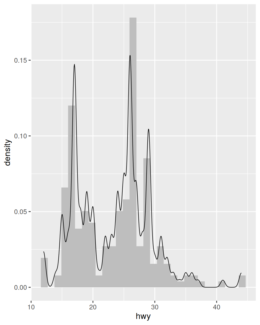
Distribution Density
ggplot(mpg) + aes(hwy, after_stat(density)) + geom_histogram(fill=NA) + geom_histogram(fill="gray", bins=10) + geom_density()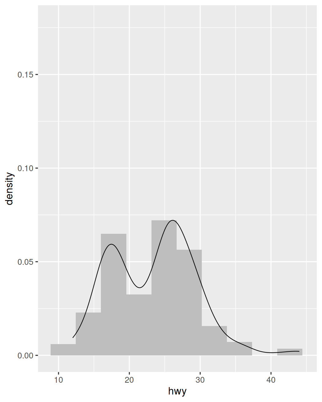
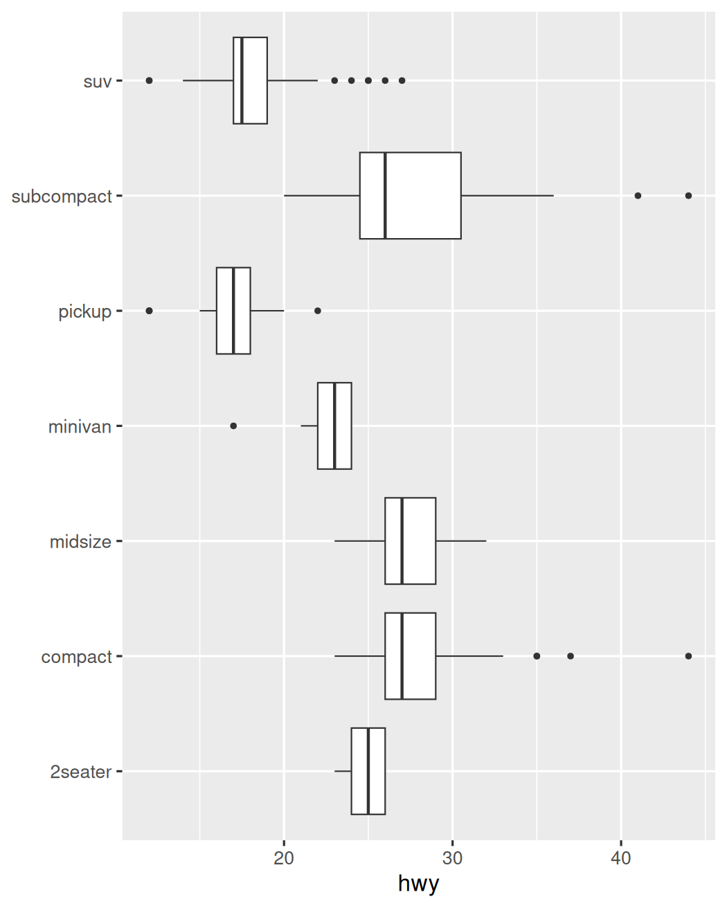
Distribution Boxplot
ggplot(mpg) + aes(hwy, reorder(class, hwy, median)) + geom_boxplot() + labs(y=NULL)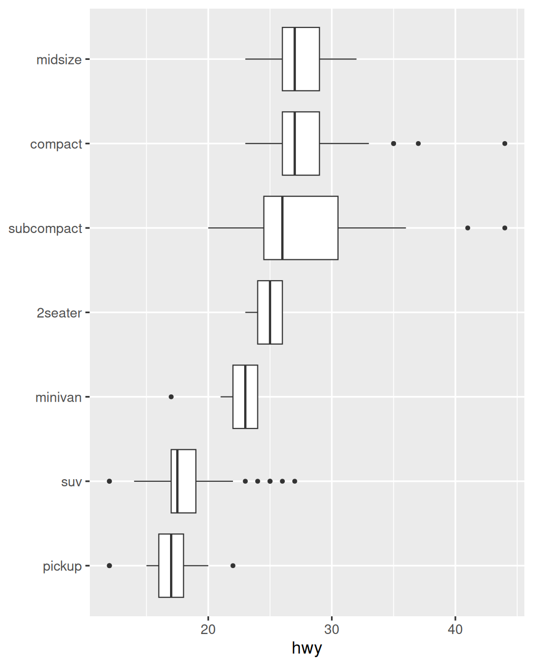
Distribution Boxplot
ggplot(mpg) + aes(hwy, reorder(class, hwy, median)) + geom_boxplot(outlier.color="red") + labs(y=NULL)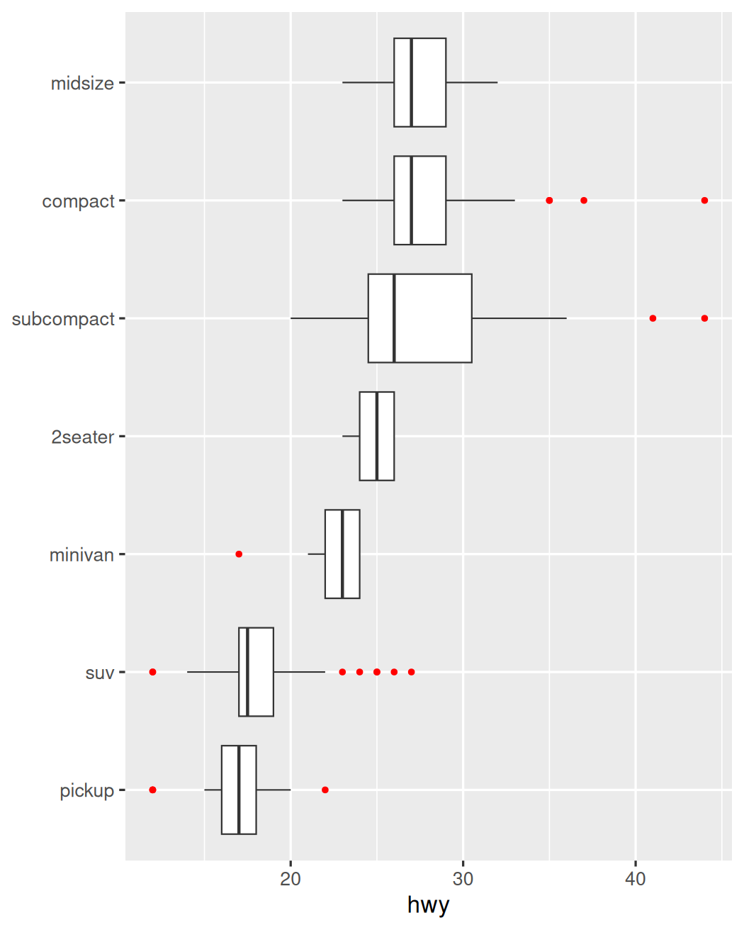
Distribution Boxplot
ggplot(mpg) + aes(hwy, reorder(class, hwy, median)) + geom_boxplot(outlier.color="red") + geom_jitter(height=0.2, alpha=0.5) + labs(y=NULL)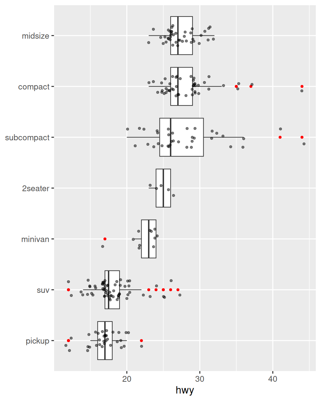
Distribution Boxplot
ggplot(mpg) + aes(hwy, reorder(class, hwy, median)) + geom_boxplot(outlier.color="red", varwidth=TRUE) + geom_jitter(height=0.2, alpha=0.5) + labs(y=NULL)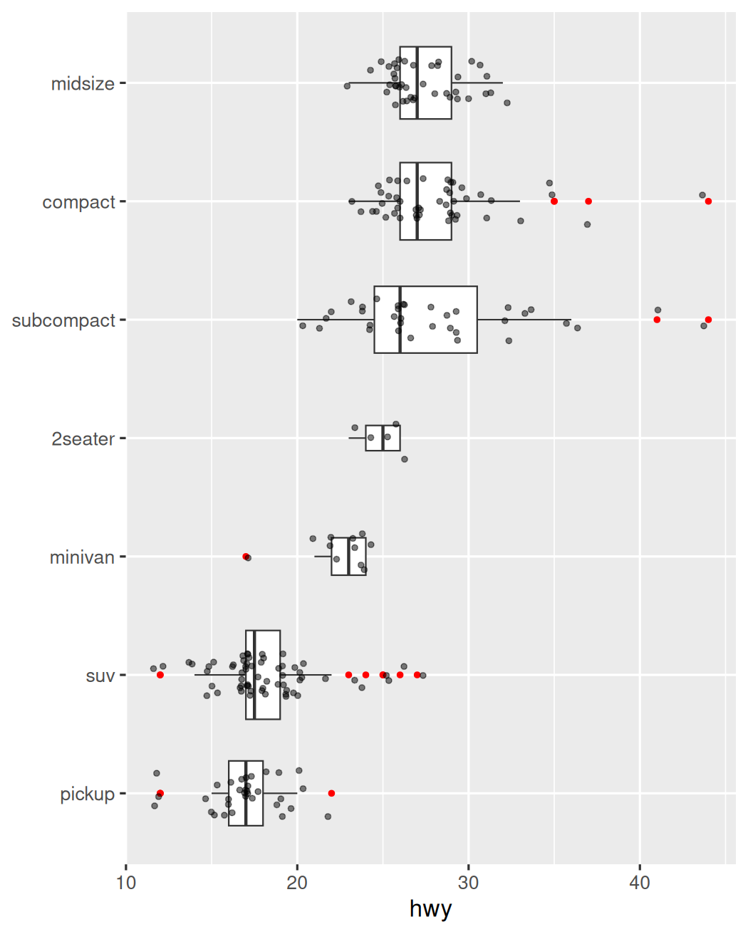
Distribution Boxplot
ggplot(mpg) + aes(hwy, reorder(class, hwy, median)) + geom_boxplot(aes(color=drv)) + labs(y=NULL) + theme(legend.position=c(1, 0), legend.justification=c(1, 0))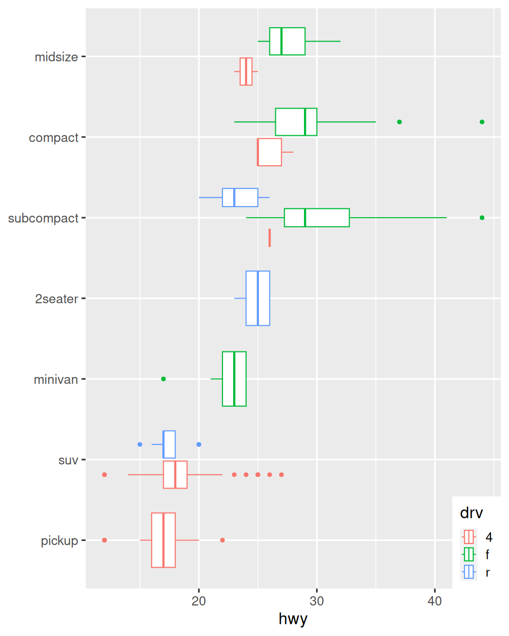
Distribution Boxplot
ggplot(mpg) + aes(hwy, reorder(class, hwy, median)) + geom_boxplot(aes(fill=drv)) + labs(y=NULL) + theme(legend.position=c(1, 0), legend.justification=c(1, 0))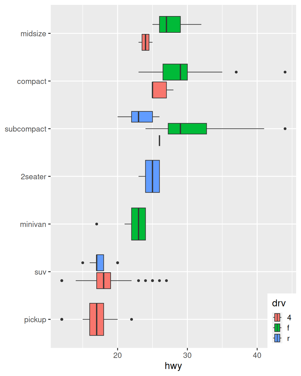
Distribution Boxplot
ggplot(mpg) + aes(hwy, reorder(class, hwy, median)) + geom_boxplot(aes(fill=drv), varwidth=TRUE) + labs(y=NULL) + theme(legend.position=c(1, 0), legend.justification=c(1, 0))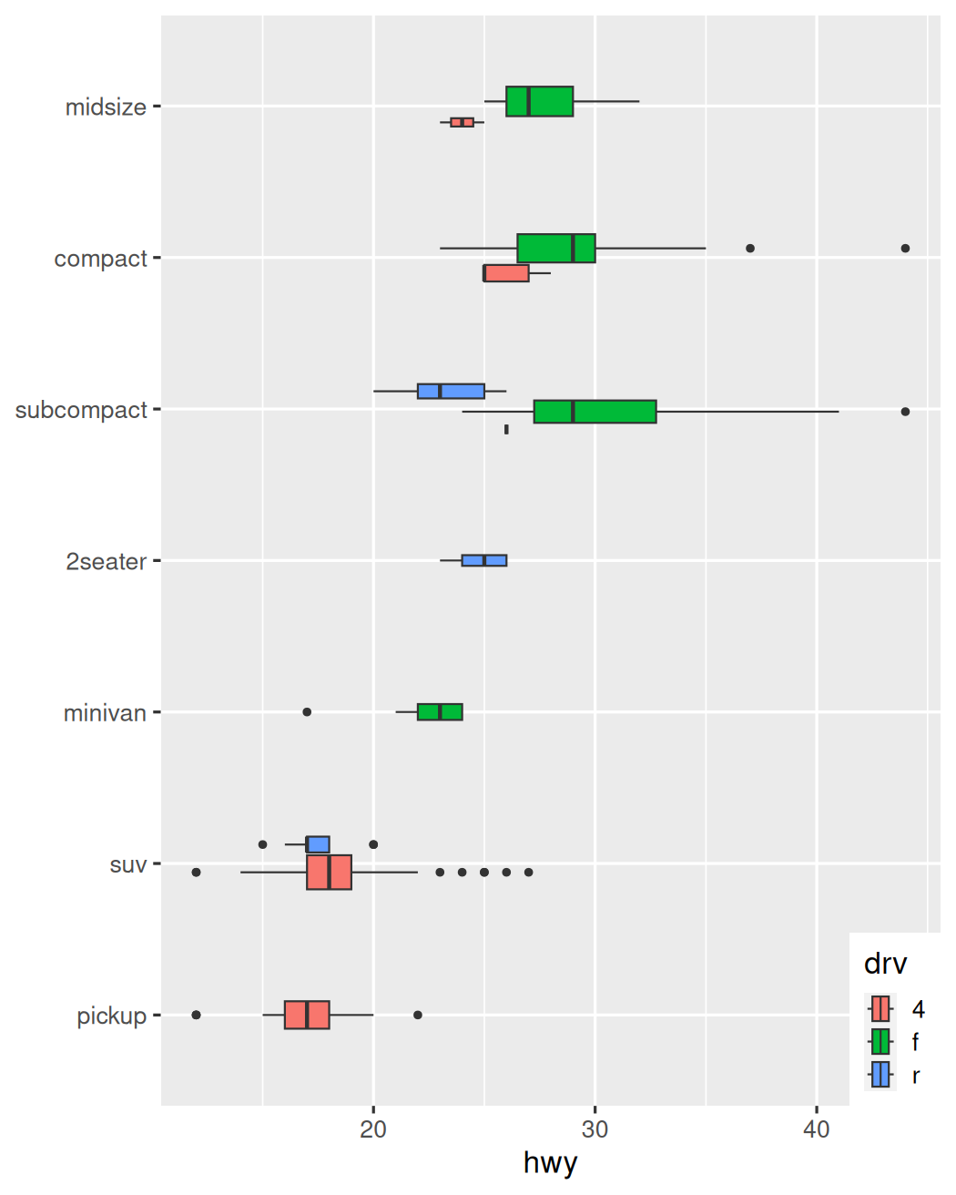
Distribution Violin
ggplot(mpg) + aes(hwy, reorder(class, hwy, median)) + geom_violin() + labs(y=NULL)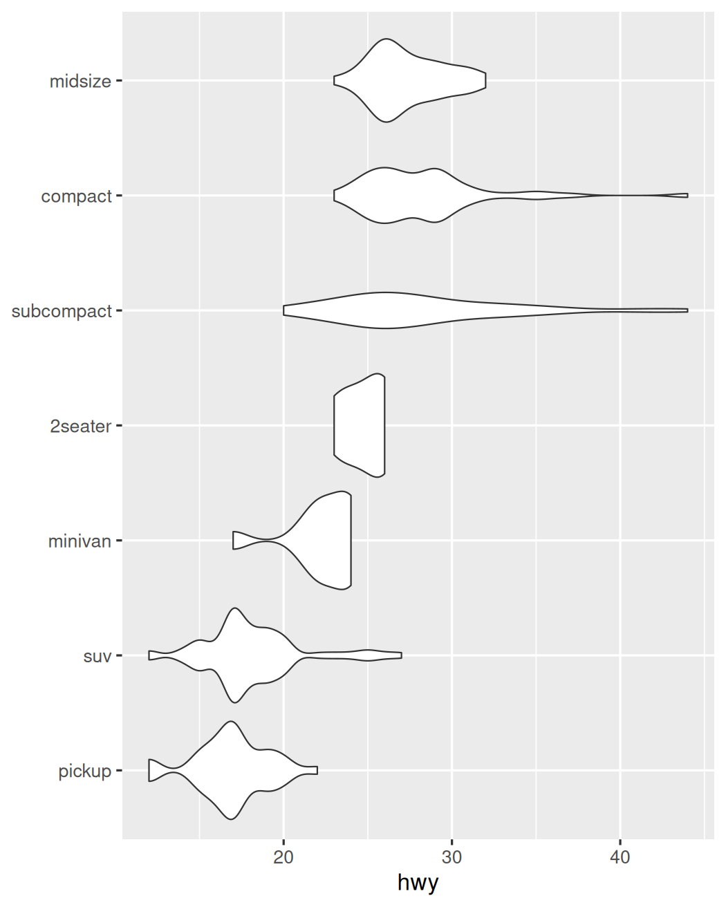
Distribution Violin
ggplot(mpg) + aes(hwy, reorder(class, hwy, median)) + geom_violin(aes(fill=class)) + labs(y=NULL) + theme(legend.position="none")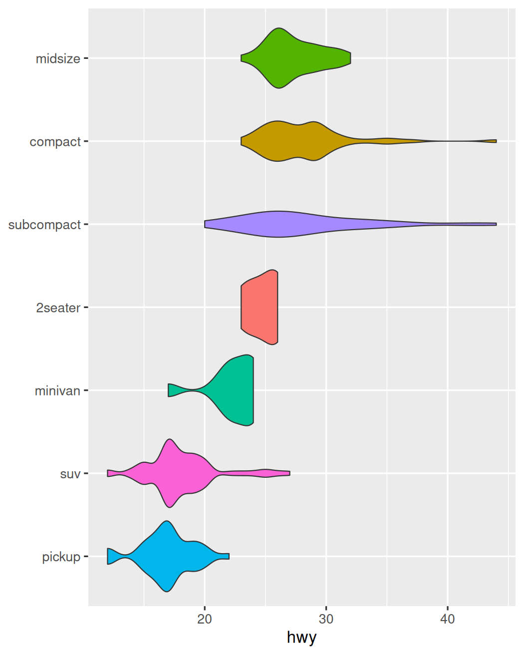
Distribution Violin
ggplot(mpg) + aes(hwy, reorder(class, hwy, median)) + geom_violin(aes(fill=class)) + scale_fill_viridis_d() + labs(y=NULL) + theme(legend.position="none")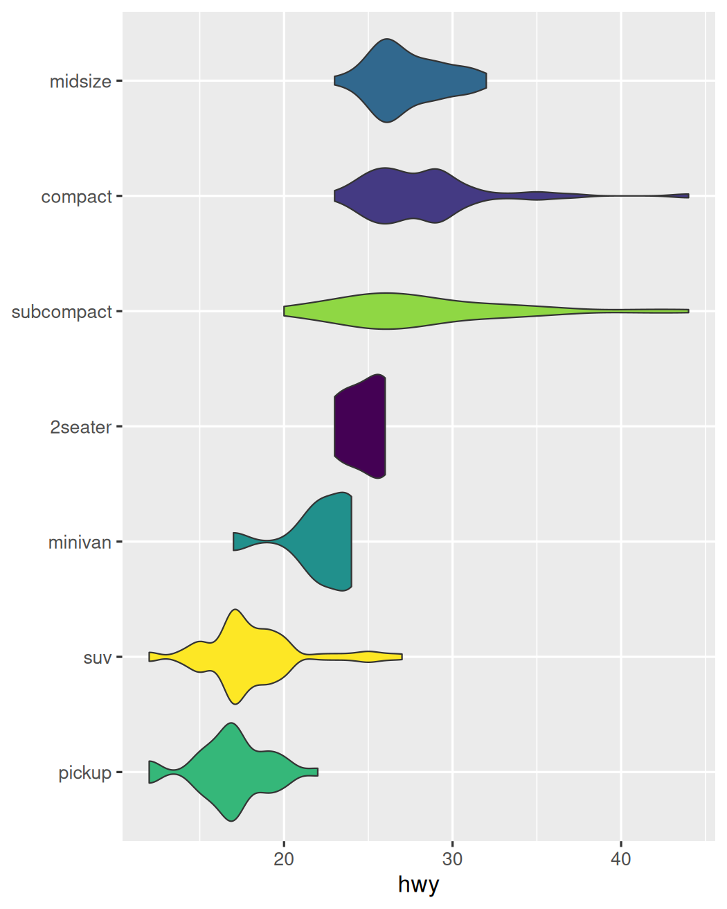
Distribution Violin
mpg |> mutate( class=reorder(class, hwy, median)) |>ggplot() + aes(hwy, class) + geom_violin(aes(fill=class)) + scale_fill_viridis_d() + labs(y=NULL) + theme(legend.position="none")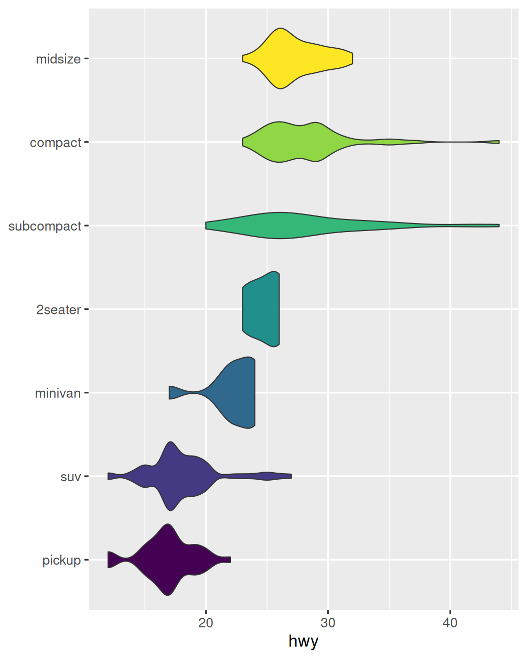
Distribution Ridgeline
mpg |> mutate( class=reorder(class, hwy, median)) |>ggplot() + aes(hwy, class, fill=class) + ggridges::geom_density_ridges() + scale_fill_viridis_d() + labs(y=NULL) + theme(legend.position="none")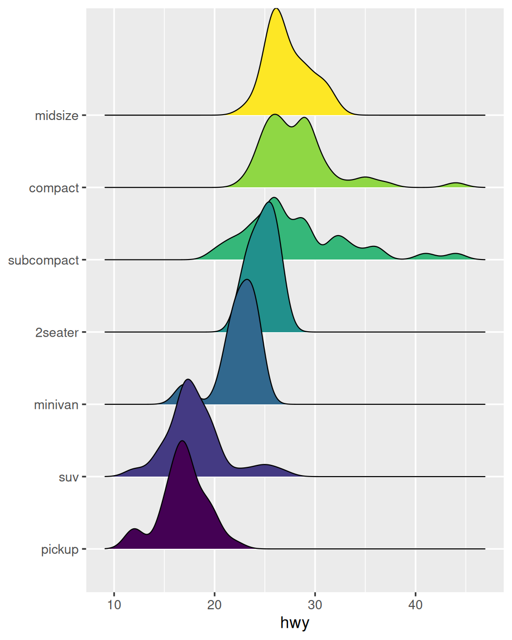
Distribution Ridgeline
mpg |> mutate( class=reorder(class, hwy, median)) |>ggplot() + aes(hwy, class, fill=after_stat(x)) + ggridges::geom_density_ridges_gradient() + scale_fill_viridis_c() + labs(y=NULL) + theme(legend.position="none")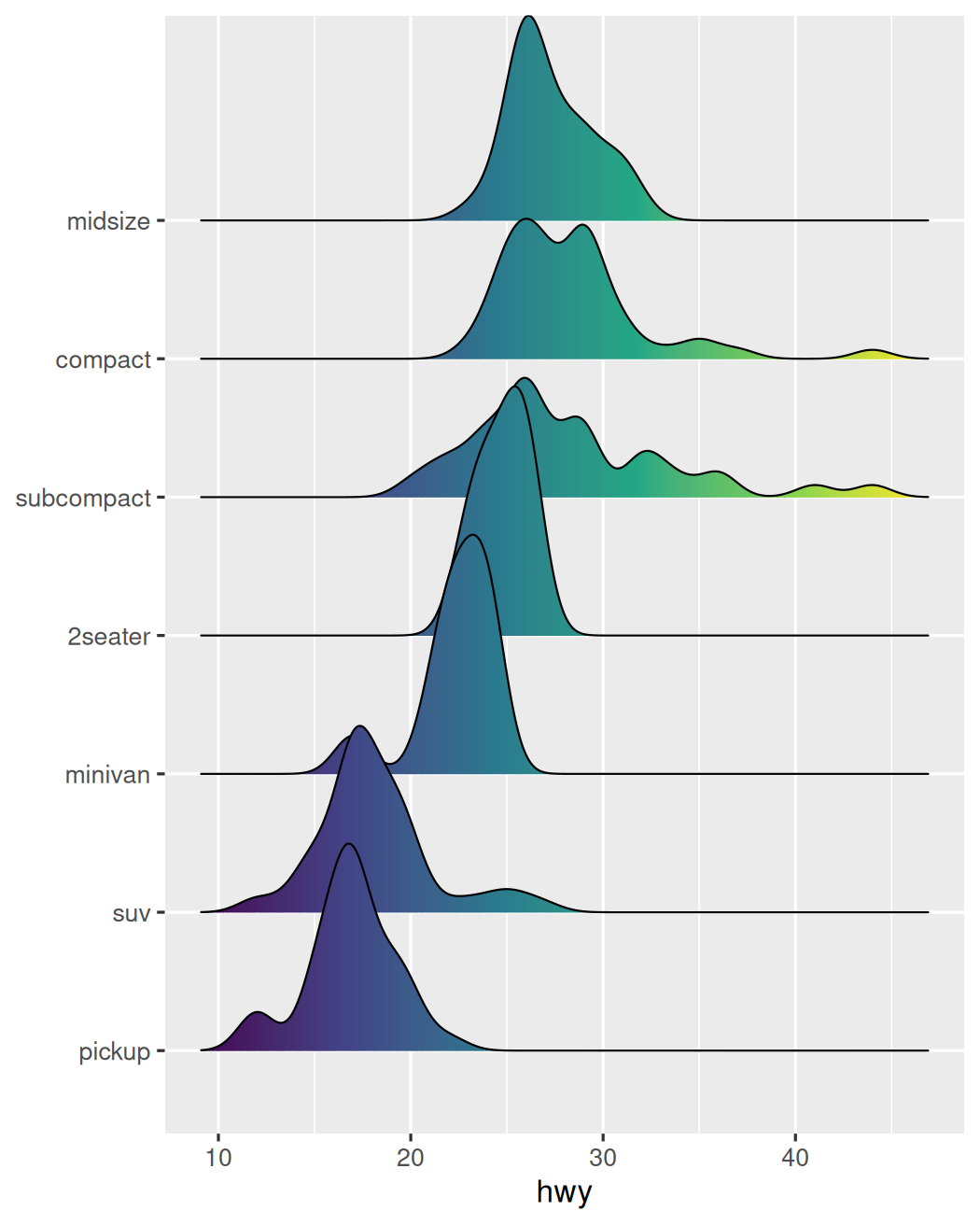
Distribution Ridgeline
mpg |> mutate( class=reorder(class, hwy, median)) |>ggplot() + aes(hwy, class, fill=after_stat(x)) + ggridges::geom_density_ridges_gradient( scale=1) + scale_fill_viridis_c() + labs(y=NULL) + theme(legend.position="none")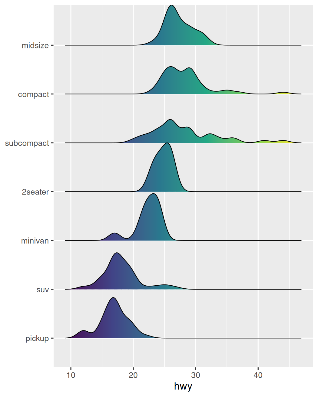
Distribution Ridgeline
mpg |> mutate( class=reorder(class, hwy, median)) |>ggplot() + aes(hwy, class, fill=after_stat(x)) + ggridges::geom_density_ridges_gradient( scale=1, quantile_lines=TRUE) + scale_fill_viridis_c() + labs(y=NULL) + theme(legend.position="none")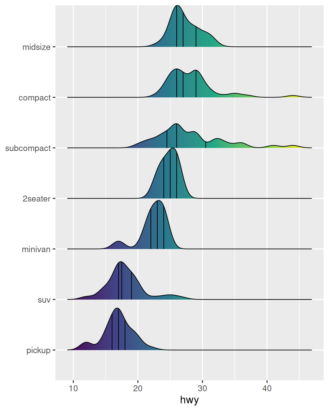
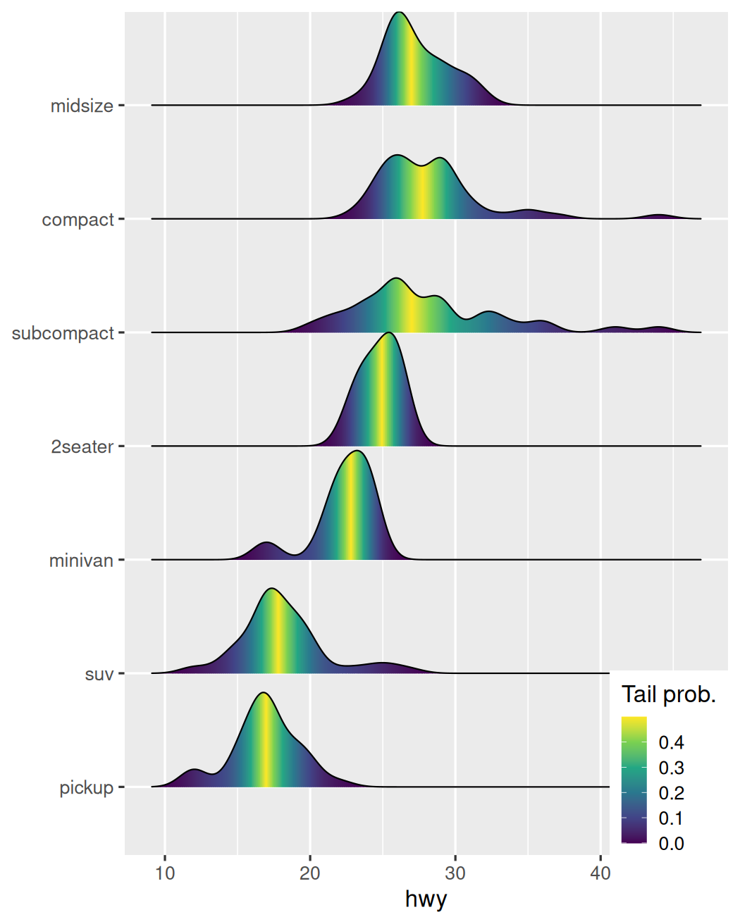
Distribution Ridgeline
mpg |> mutate( class=reorder(class, hwy, median)) |>ggplot() + aes(hwy, class, fill=0.5 - abs( 0.5 - after_stat(ecdf))) + ggridges::geom_density_ridges_gradient( scale=1, calc_ecdf=TRUE) + scale_fill_viridis_c("Tail prob.") + labs(y=NULL) + theme(legend.position=c(1, 0), legend.justification=c(1, 0))