Polio Vaccine in the US
The polio vaccine is an important tool in the fight against polio, a highly infectious disease that can cause paralysis and death. Polio is caused by a virus that spreads through contaminated food and water and can attack the nervous system, leading to paralysis in some cases.
The first polio vaccine was developed in the 1950s by Dr. Jonas Salk. The first mass vaccination campaign against polio was launched in April of 1995 in the US. The oral polio vaccine was introduced in the US in 1961 and became the primary vaccine used for routine polio vaccination in the US in the 1970s.
Since the introduction of the polio vaccine in the US, the incidence of polio has decreased dramatically. The last case of wild poliovirus was reported in 1979, and the disease has been considered eradicated in the US since 2000. The success of the polio vaccine in the United States and around the world has been one of the greatest public health achievements of the 20th century.
Original Plot - WSJ
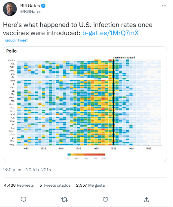
The original plot was created by Tynan DeBold and Dov Friedman and published in February 2015 in an article in the Wall Street Journal, and is part of a series of graphics showing the effect of vaccines on different diseases such as measles, heaptitis A, mumps, pertussis, rubella, among others.
The visualization was so good that it had a great impact on social networks…
Reproducing de Original Plot
library(readr)
library(tidyverse)
library(tibble)
library(ggplot2)
library(lubridate)
library(forcats)
library(scales)
library(viridis)
library(grDevices)
library(plotly)
library(systemfonts)
library(patchwork)
library(cowplot)
library(RColorBrewer)
library(showtext)
Data Source –> tycho.pitt.edu
The data in the original plot is from tycho.pitt.edu, a research project aimed at improving the standards, machine readability and availability of global health data, which is sponsored by the University of Pittsburgh in the US.
However, when we consulted the historical records of polio cases registered in the USA, we found that there are several polio viruses: Acute nonparalytic poliomyelitis, Acute paralytic poliomyelitis, Acute poliomyelitis.
The original plot does not specify which of the three viruses it refers to, so it was decided to use the information of all the viruses that make up the polio disease.
Acute nonparalytic poliomyelitis
Polio  <- read_csv("tycho_20221212-145444.csv",
                    col_types = cols_only(Admin1Name = col_guess(),
                                          PeriodStartDate = col_guess(),
                                        CountValue = col_guess()))%>%
  mutate(PeriodStartDate = ymd(PeriodStartDate)) %>%
  arrange(Admin1Name, by="name") %>%
  count(Admin1Name,lubridate::floor_date(PeriodStartDate, "year")) %>%
  rename(State =Admin1Name,
         Date = `lubridate::floor_date(PeriodStartDate, "year")`,
         Cases = n)
Acute paralytic poliomyelitis
Polio1 <- read_csv("tycho_20221215-094815.csv",
                   col_types = cols_only(Admin1Name = col_guess(),
                                         PeriodStartDate = col_guess(),
                                         CountValue = col_guess()))%>%
  mutate(PeriodStartDate = ymd(PeriodStartDate)) %>%
  arrange(Admin1Name, by="name") %>%
  count(Admin1Name,lubridate::floor_date(PeriodStartDate, "year")) %>%
  rename(State =Admin1Name,
         Date = `lubridate::floor_date(PeriodStartDate, "year")`,
         Cases = n)
Acute poliomyelitis
Polio2 <- read_csv("tycho_20221215-095240.csv",
                   col_types = cols_only(Admin1Name = col_guess(),
                                         PeriodStartDate = col_guess(),
                                         CountValue = col_guess()))%>%
  mutate(PeriodStartDate = ymd(PeriodStartDate)) %>%
  arrange(Admin1Name, by="name") %>%
  count(Admin1Name,lubridate::floor_date(PeriodStartDate, "year")) %>%
  rename(State =Admin1Name,
         Date = `lubridate::floor_date(PeriodStartDate, "year")`,
         Cases = n)
Cleaning Data
We now have the three clean data sets with the number of cases by State and by date.
Next we will merge the three data sets into one and then add up all the cases so that we have a consolidated file.
Abb <- read_delim("US State Abbreviations.csv",
    delim = ";", escape_double = FALSE, trim_ws = TRUE)

Poliojoint <- full_join(Polio2, Polio1, by = c("State" = "State", "Date" ="Date"))

Poliojoint1 <- full_join(Poliojoint, Polio, by = c("State" = "State", "Date" ="Date"))

Poliojoint2 <- left_join(Poliojoint1, Abb, by = c("State" = "States"))

Polio_sum <- Poliojoint2 %>%  mutate_at(c('Cases.x', 'Cases.y', "Cases"), as.numeric) %>%
  mutate(sum_cases = rowSums(across(where(is.numeric)), na.rm=T), .keep = "unused") %>%
  filter(Date >= '1928-01-01') %>% rename(States = Abb) %>% select(-State)
Colors
To copy the colors of the original plot, I used the website “html-color-codes.info” which allows to upload the image and obtain all the codes present in the image.
cols <- c(colorRampPalette(c("#e7f0fa", "#c9e2f6", "#95cbee", "#0099dc","#BAC843",
                            "#4ab04a", "#ffd73e", "#eec73a", "#e29421", "#e29421",
                            "#f05336","#ce472e"),bias=1)(11))
Original Plot
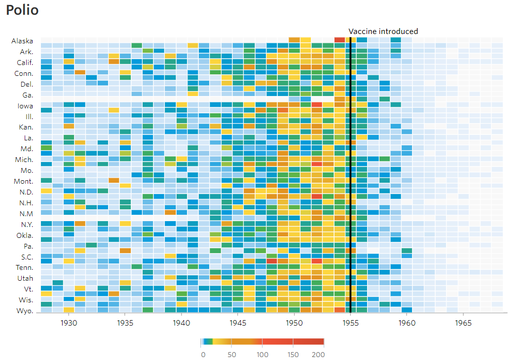
The original graph is a heat map showing the number of polio cases reported in each U.S. state over time. For that reason, the x-axis will be the US states, and the y-axis will be the years and the plot will be filled by the number of cases.
As this is a heatmap, to add rectangles we will use the geom_tile function. Additionally, the original plot has white spaces between the rectangles, so we are going to specify this inside the function.
p <- p + geom_tile(colour="white", lwd = 0.2, linetype = 1)
p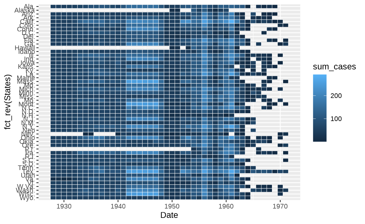
Next we are going to use the scale_fill_gradientn() function to set the fill color of the rectangles in a continuous gradient. The colors argument specifies the colors to use in the gradient, for which we will use the color palette defined above (“cols”). Then we define the minimum and maximum limits, which correspond to the minimum and maximum number of polio cases in a year. We include the breaks at which the gradient should change color, and specify the labels for these values.
Additionally, we use the guide argument to control the appearance of the color bar displayed next to the plot. For this purpose we define gradient marks, number of intervals to use for the gradient, and the color bar height and width arguments, respectively.
 p <- p+theme_minimal()+
  scale_fill_gradientn(colours=cols,limits=c(0, 300),
                       breaks=seq(0, 300, by=50),
                       labels=c("0", "50", "100", "150", "200", "250", "300"),
                       guide=guide_colourbar(ticks=T,
                                             nbin=50,
                                             barheight=.6,
                                             label=T,
                                             barwidth=8,
                                             ticks.colour= "grey",
                                             ticks.linewidth = 0.5))
p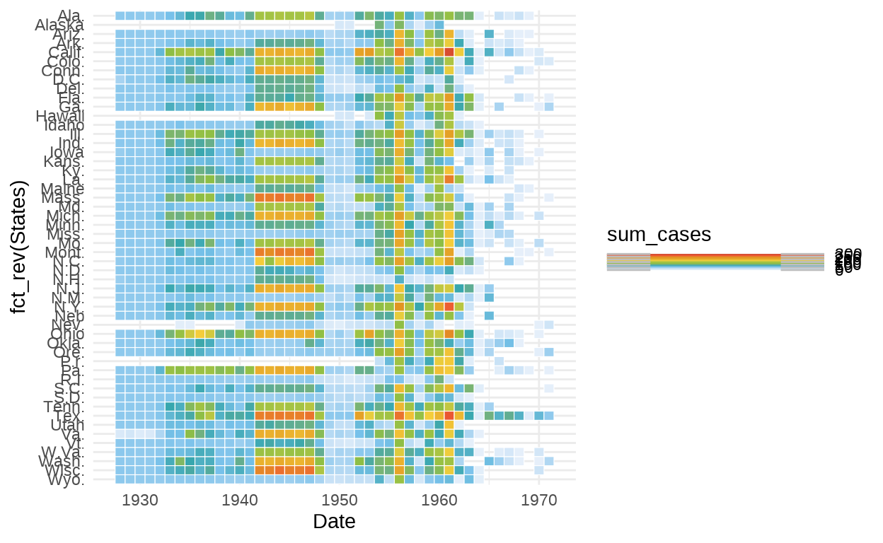
We use scale_x_date() function to set the scale of the x-axis to a date format. Then we need to specify the amount of space to add around the data. A value of c(0,0) means no space is added.
The breaks argument specifies the positions of the tick marks on the x-axis. In this case, the seq() function is used to generate a sequence of dates at 5-year intervals from 1930 to 1965.The date_labels argument specifies the format to use for the labels of the tick marks. In this case, the format “%Y” is used, which displays the year in four digits.
p <- p+ scale_x_date(expand=c(0,0),
                     breaks = (seq(ymd("1930-01-01"), ymd("1965-01-01"),
                                   by = "5 years")),
                     date_labels = "%Y")
p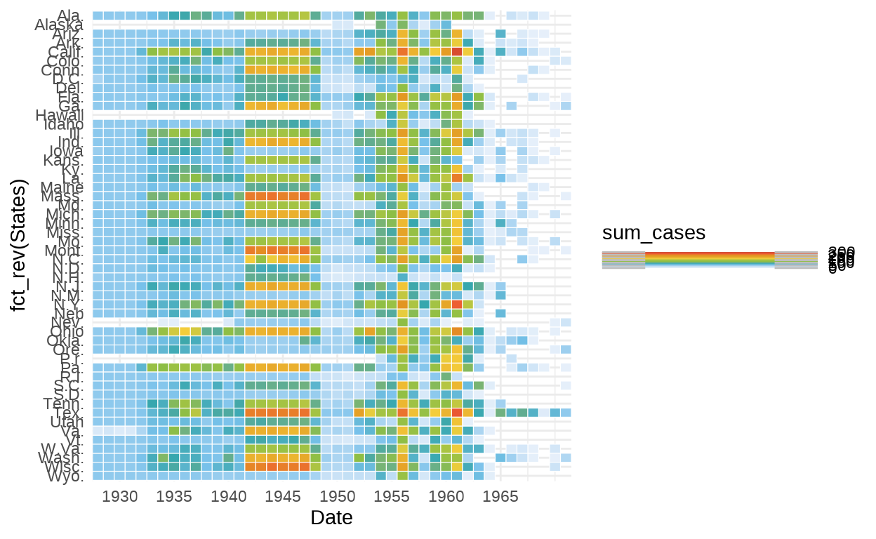
To include the line indicating the time at which the vaccine was introduced, we will use the function geom_segment(). In this case, the line segment will start at the date “1955-01-01” and end at the same date, so it will be a vertical line.
 p <- p + geom_segment(x=as.Date("1955-01-01"), xend=as.Date("1955-01-01"),
                       y=0,
                       yend=52.5,
                       size=.9)
p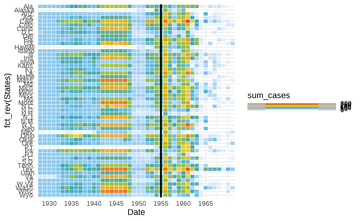
Now we want to find the right font. For that we use the website “What the Font” which tells us the font used. However, the exact font has a high cost and is not available. Therefore, we searched Google fonts for the closest possible match, and found the Tajawal family font.
To use this font we make use of the “showtext” package, then we select the Google font we want using font_add_google(“Tajawal”), and then we call showtext_auto() to indicate that showtext is going to be automatically invoked to draw text whenever the plot is created.
font_add_google("Tajawal")
showtext_auto()
Now we use different functions to modify the appearance of the chart to make it resemble the original. The labs() function is used to remove the x-axis, y-axis and fill legend labels. The ggtitle() function is used to set the chart title. The theme() function is used to customize various aspects of the chart appearance, for example the aspect ratio, legend position, and axis labels and markings.
 p <-  p + labs(x="", y="", fill="")+
  ggtitle("Polio") +
  theme(    legend.position= "bottom",
        legend.direction="horizontal",
        legend.text=element_text(colour="grey20"),
        axis.text.y=element_text(size=8, family="Tajawal",
                                 hjust=1),
        axis.text.x=element_text(size=6),
        axis.ticks.y=element_blank(),
    axis.ticks.x=element_line(color = "grey50", size = 0.5),
    axis.line.x =element_line(color = "grey50", size = 0.5),
        panel.grid=element_blank(),
        title=element_text(hjust=-.07, face="bold", vjust=1,
                           family="Tajawal"),
        text=element_text(family="Tajawal"))
p
Finally, we add a label with the text “Vaccine introduced” to the plot at the specified x and y coordinates, using the specified font size and font family. The label will be aligned top left and the aspect ratio of the plot will be set.
  p <- p+ annotate("text", x=as.Date("1955-01-01"), y=55, label="Vaccine introduced",
           vjust=1, hjust=0, size=I(3), family="Tajawal")
p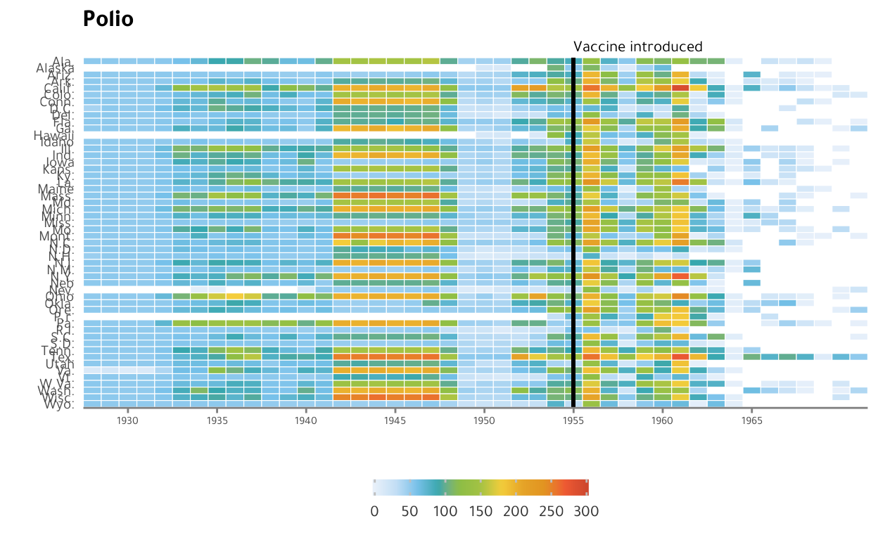
As can be seen, the plots are not identical because the data set used is not the same.
An attempt was made to use the same data set to replicate the original plot as closely as possible, but the same dataset was not found. For this reason, it was decided to use the three datasets with the three viruses that make up the polio, resulting in a slightly different plot.
In this version, we can see that after the introduction of the vaccine in 1955 there was no drastic decrease in the number of cases, but on the contrary there was a slight increase in 1956. In addition, we can see that the number of cases actually dropped significantly after 1961, which coincides with the date when an improved version of the vaccine was introduced in the US.
Improved plot
It is a great challenge to make an improvement of a plot so well done and with so many recognitions. In fact, I personally consider that the original plot is the best way to visualize the effect of a vaccine in reducing the number of positive cases of contagion.
Therefore, I am not going to propose a new plot. Instead, I am going to improve the original plot by adding more useful information.
First, as the most important thing is to see the effect of the vaccine, let’s reduce the number of years exposed. To do this we will start in the year 1940 and end in the year 1970. For this purpose we will reduce the dataset.
Polio_sum1 <- Polio_sum %>% filter(Date >= "1940-01-01" & Date <= "1966-01-01")

p1 <- Polio_sum1 %>% ggplot() +
  aes(x=(Date), y=fct_rev(States),fill=sum_cases) +
  geom_tile(colour="white", lwd = 0.2, linetype = 1)+
  theme_minimal()+
  scale_x_date(expand=c(0,0),
               breaks = (seq(ymd("1930-01-01"), ymd("1970-01-01"),
                             by = "5 years")), date_labels = "%Y")+
  labs(x="", y="", fill="")+
  theme(aspect.ratio = 6.5/12.5,
        legend.position= "bottom",
        legend.direction="horizontal",
        legend.text=element_text(colour="grey50"),
        axis.text.y=element_text(size=6, family="Tajawal"),
        axis.text.x=element_text(size=6),
        axis.ticks.y=element_blank(),
    axis.ticks.x=element_line(color = "grey50", size = 0.5),
    axis.line.x =element_line(color = "grey50", size = 0.5),
        panel.grid=element_blank(),
        title=element_text(hjust=-.07, vjust=1,
                           family="Tajawal"),
        text=element_text(family="Tajawal"))
I want to change the palette color to a color with more visual impact. That is why I want to choose a palette that makes it easier to see the years with the highest polio cases. That’s why I chose the YlGnBu palette from the RColorBrewer package, which gives a very interesting effect.
p1 <- p1 + scale_fill_gradientn(colours=brewer.pal(n=9, "YlGnBu"),limits=c(0, 300))
p1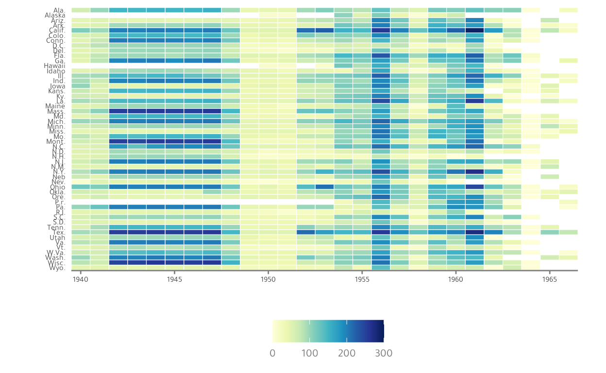
I want also to include a new line distinguishing between the two types of vaccines that were introduced in the U.S.: the injected vaccine invented and licensed in 1955 by Jonas Salk, and the improved oral vaccine invented by Albert Sabin that was introduced in 1961, targeting all types of polio.
This shows that it was only after the introduction of the second vaccine in 1961 that there was a real decrease in polio cases in the United States.
p1 <- p1 + geom_segment(x=as.Date("1955-01-01"), xend=as.Date("1955-01-01"),
               y=0, yend=52.5, size=.9, color="grey50", alpha=0.5)+
  annotate("text", x=as.Date("1952-01-01"), y=56, label="First vaccine",
           vjust=1, hjust=0, size=I(3), family="Tajawal", color="grey50")+
   geom_segment(x=as.Date("1961-01-01"), xend=as.Date("1961-01-01"),
                y=0, yend=52.5, size=.9, color="grey50", alpha=0.5)+
  annotate("text", x=as.Date("1960-01-01"), y=56, label="Second vaccine",
           vjust=1, hjust=0, size=I(3), family="Tajawal", color="grey50")
p1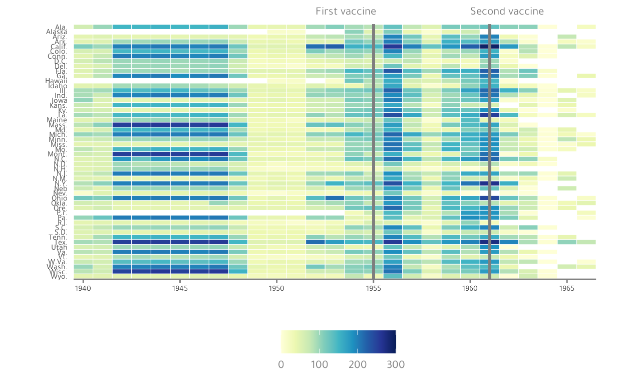
Now, we will introduce a more explanatory title and subtitle about the plot.
p1 <- p1 + labs(title="Effect of the introduction of the two polio vaccines in the US",
       subtitle=paste("The heat map represents a visualization of the positive cases of Polio",
                      "in the USA during the years 1928 and 1971 for the three existing virus",
                      "\ntypes (Nonparalytic poliomyelitis, Paralytic poliomyelitis, poliomyelitis),",
                      "where the decrease of positive cases due to the introduction of the",
                      "\ntwo vaccines can be clearly seen."))+
  theme(plot.subtitle=element_text(size=6), plot.title=element_text(size=10))
p1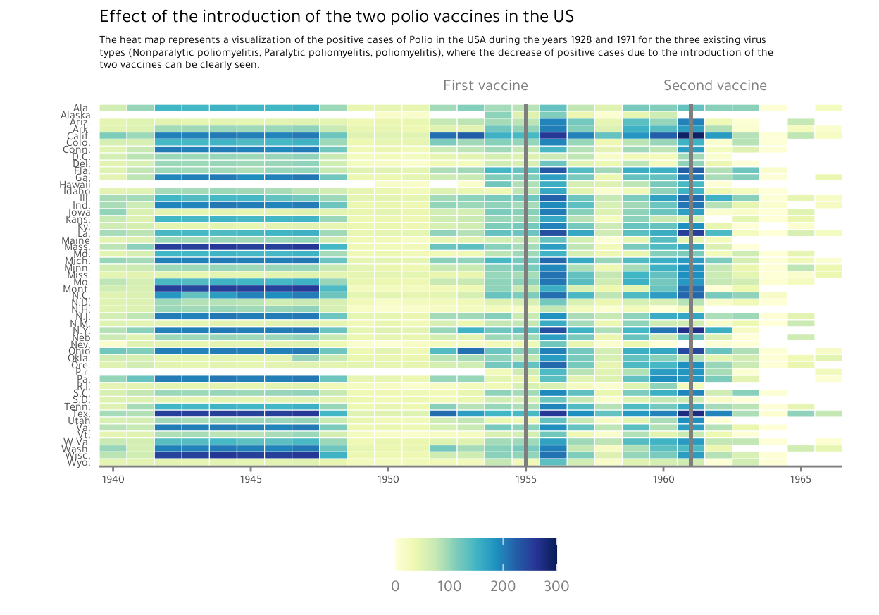
Now I want to include to the plot the number of cases presented in each of the states in order to easily visualize which of the states was the most affected by the polio virus.
In that sense, we are going to modify the dataset to obtain the cases presented in each state during the years 1928 and 1971.
Next, we are going to make a Barplot using the geom_col function, filling the bars with the colors representing the number of cases per state.
casebars <- ggplot(Casesxstate) +
  aes(x=total_cases, y=fct_rev(States), fill=total_cases)+
  geom_col(show.legend=FALSE)+
  theme_minimal()+
  scale_fill_gradientn(colors = brewer.pal(n=9, "YlGnBu"),
                       limits=c(1000, 6000))+
  scale_x_continuous()+
  theme( aspect.ratio = 3/1, panel.grid=element_blank(),
    axis.title.y=element_blank(),
    axis.title.x=element_blank(),
    axis.line.y=element_blank(),
    axis.text.y=element_blank(),
        axis.ticks.y=element_blank(),
    axis.text.x=element_text(size=6, colour="grey50"),
    axis.ticks.x=element_line(color = "grey50", size = 0.5),
    axis.line.x =element_line(color = "grey50", size = 0.5))
casebars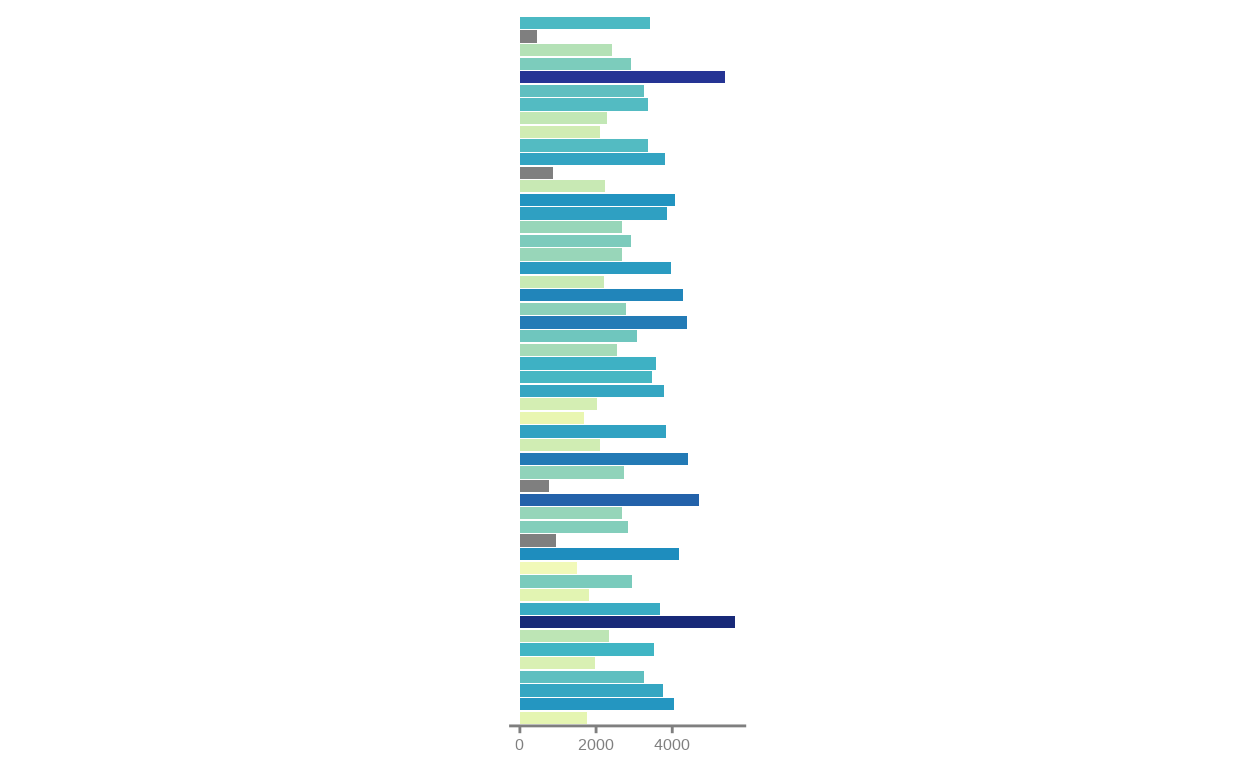
Next, we will use the patchwork package to assemble different plots. In our case, we are going to use the “inset_element” function to assemble the original plot with the new plot so that they are in the same plot. Let’s see.
p1+ inset_element(casebars,
                       left=0.95,
                       bottom=-0.1,
                       right=1.22,
                       top=0.965,
                       align_to="panel",
                  clip = TRUE)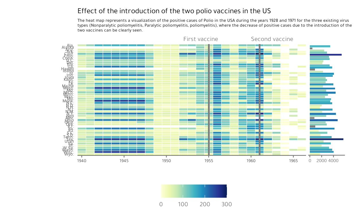
With these improvements to the plot we can more easily see the change of colors in relation to the number of polio cases, we can see the effect of the introduction of the second vaccine in the US and finally we can see the states that suffered the most from Polio during the years recorded.
In conclusion, this plot uses everything that a heat map is good for as it provides an initial view of the data and allows us to explore the information in a wide visual range. Additionally, it allows you to easily analyze the data, which allows you to find patterns and trends.
