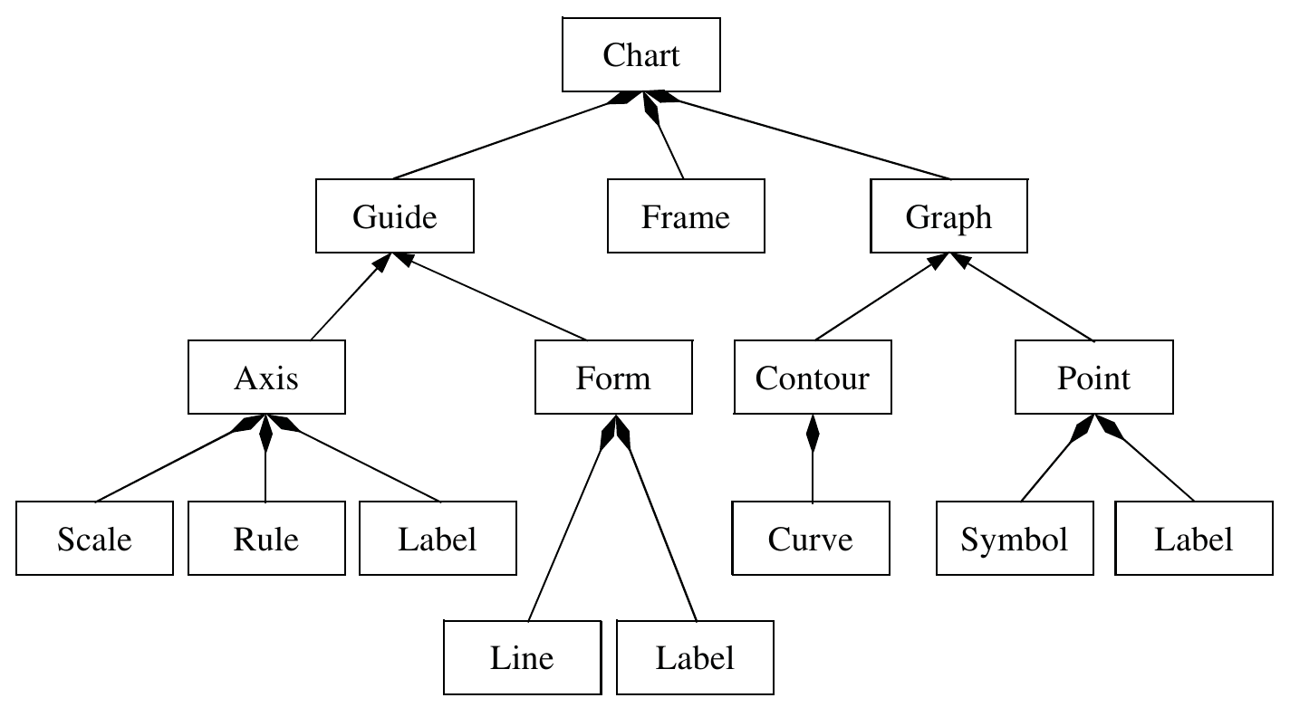
An Object-Oriented Graphics System
An Object-Oriented Graphics System
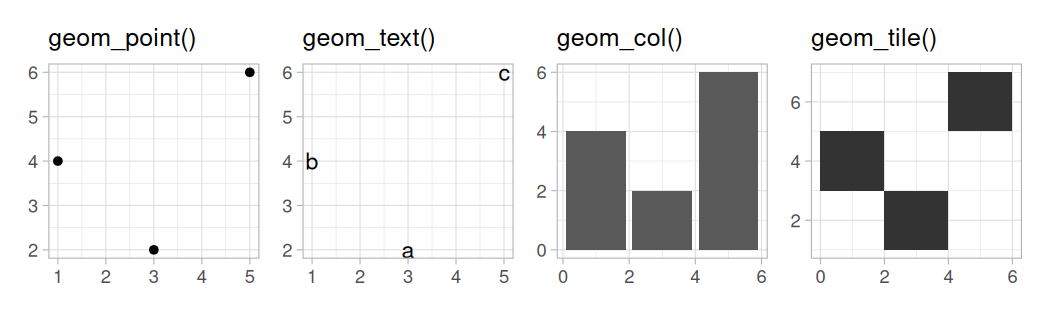
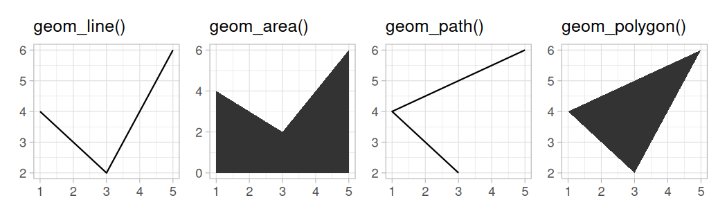
Individual Geoms
- Two dimensional: require
xandy, understandcolorandsize. - Some of them can be
filled.
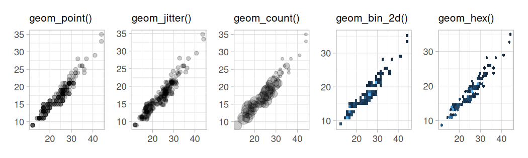
Collective Geoms
- Dealing with point overplotting
| Geom | Result | Details |
|---|---|---|
geom_jitter()geom_count()geom_bin_2d()geom_hex() |
geom_point(), but adds some jitter to each point.Maps the count of overlapping points to size.Maps the count of rectangles to fill.Same, but using hexagons. |
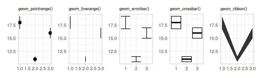
Collective Geoms
- Dealing with uncertainty
| Geom | Result | Details |
|---|---|---|
geom_pointrange()geom_linerange()geom_errorbar()geom_crossbar() |
Various ways of representing a vertical intervals defined by x, ymin and ymax. |
|
geom_ribbon() |
Special case of geom_area() with ymin too. |
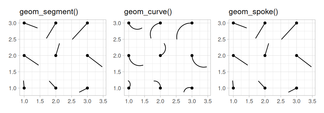
Collective Geoms
- Arbitrary segments
| Geom | Result | Details |
|---|---|---|
geom_segment()geom_curve()geom_spoke() |
Straight line between points (x, y) and (xend, yend).Same, but curved line. Polar parametrization of geom_segment(). |
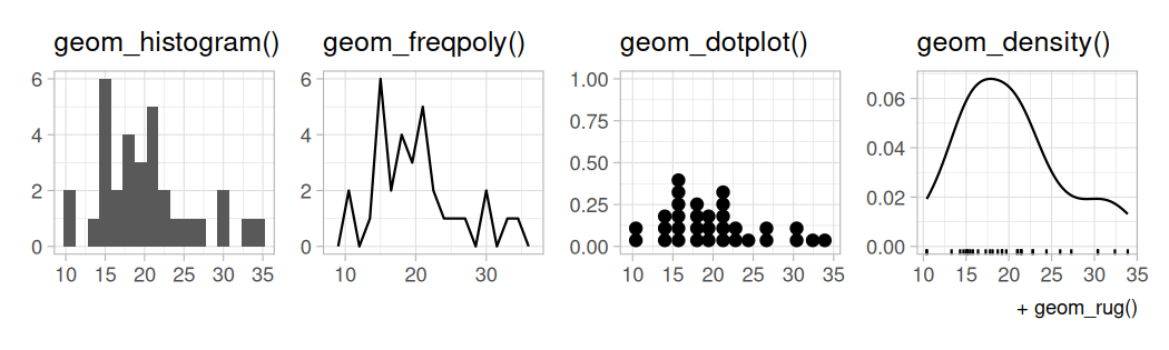
Collective Geoms
- Distributions
| Geom | Result | Details |
|---|---|---|
geom_histogram()geom_freqpoly()geom_dotplot() |
histogram | Distribution of a continuous variable by bins. To display the counts with lines instead. Histograms of stacked dots. |
geom_density() |
density plot | Smoothed version of the histogram. |
geom_rug() |
Draws ticks for marginal distributions. |
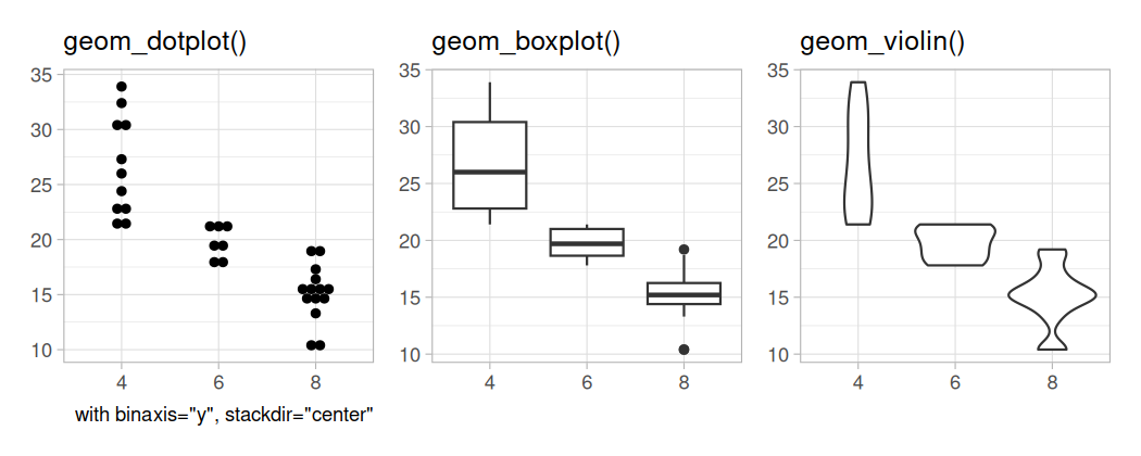
Collective Geoms
- Boxplots
| Geom | Result | Details |
|---|---|---|
geom_boxplot()geom_violin() |
boxplot | Compact display of the distribution of a continuous variable. Mirrored density, displayed as a boxplot. |
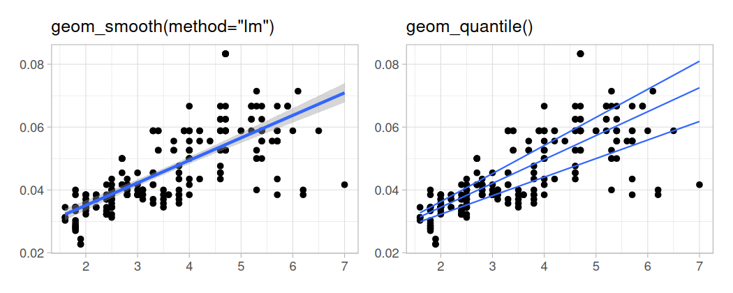
Collective Geoms
- Smoothing lines
| Geom | Result | Details |
|---|---|---|
geom_smooth()geom_quantile() |
Fits a model and draws a smoothing line. Fits a quantile regression and draws the quantiles. |
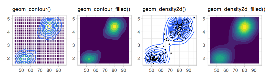
Collective Geoms
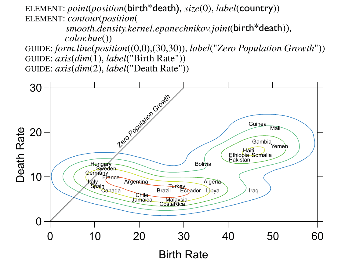
- Contours
| Geom | Result | Details |
|---|---|---|
geom_contour()geom_contour_filled()geom_density_2dgeom_density_2d_filled() |
contour plot | 2D contours of 3D surfaces of regular x, y.Filled version. 2D contours after computing the density. Filled version. |
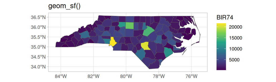
Collective Geoms
- Maps
| Geom | Result | Details |
|---|---|---|
geom_map()geom_sf()geom_sf_text()geom_sf_label() |
map | Old way to plot polygons as a map. Current recommended way via sf.Similar to geom_text() but for sf.Similar to geom_label() but for sf. |
Geom vs. Stat
ggplot(mpg, aes(displ, hwy)) + geom_point(stat="identity")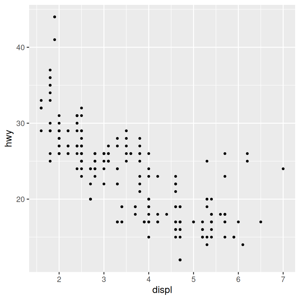
ggplot(mpg, aes(displ, hwy)) + stat_identity(geom="point")
Geom vs. Stat
ggplot(mpg, aes(hwy)) + geom_bar(stat="count")
ggplot(mpg, aes(hwy)) + stat_count(geom="bar")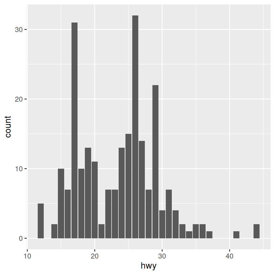
Geom vs. Stat
ggplot(mpg, aes(displ, hwy)) + geom_smooth(stat="smooth")
ggplot(mpg, aes(displ, hwy)) + stat_smooth(geom="smooth")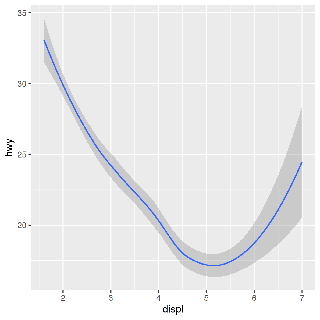
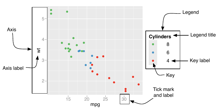
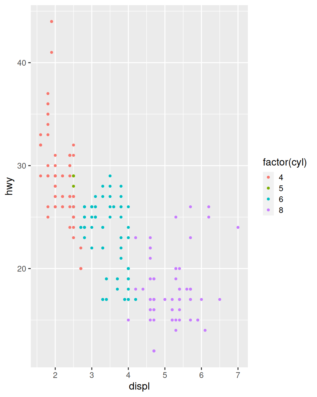
Scale Specification
A scale is a procedure that performs the mapping of data attributes into channels (position, color, size...):
sets the limits;
sets an optional transformation (without modifying the data);
sets a guide.
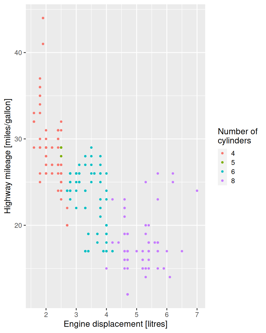
A guide allows us to revert the procedure and recover the data:
an axis or a legend, depending on the channel;
has a name, breaks, labels...
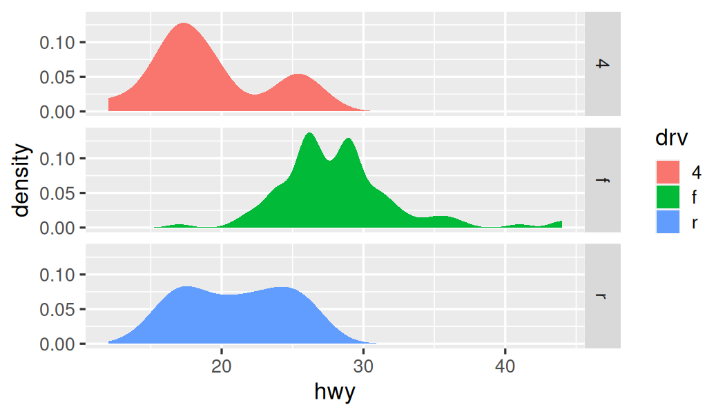
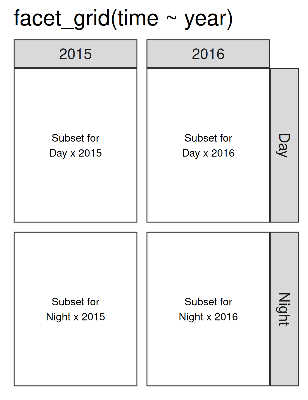
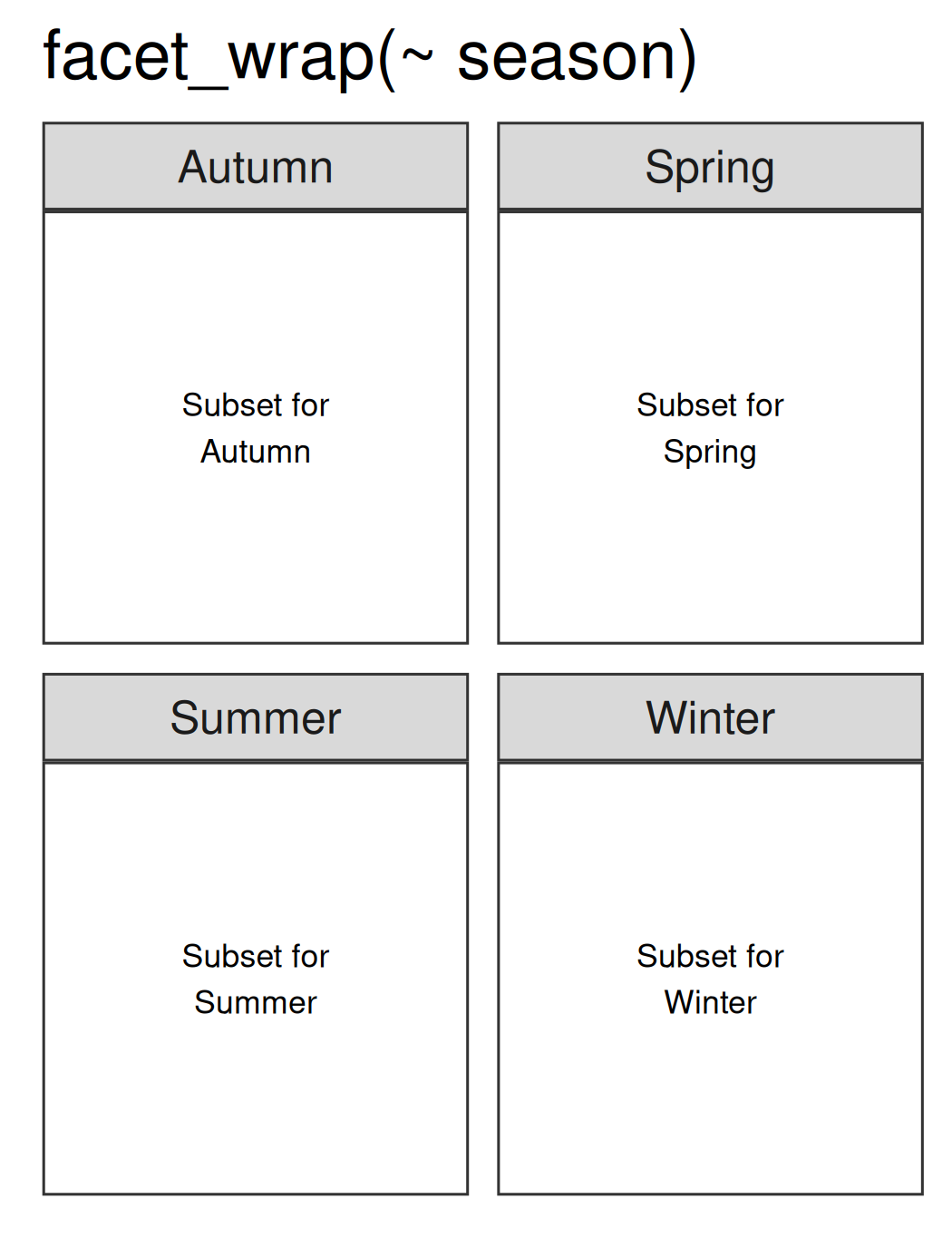
Facet Specification
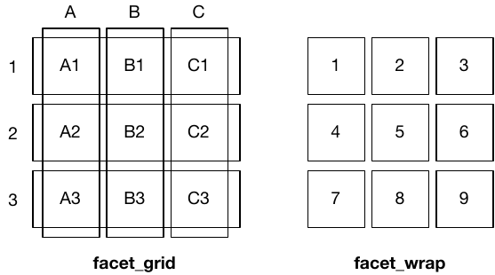
Facet Specification
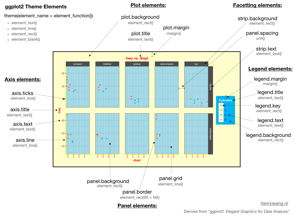
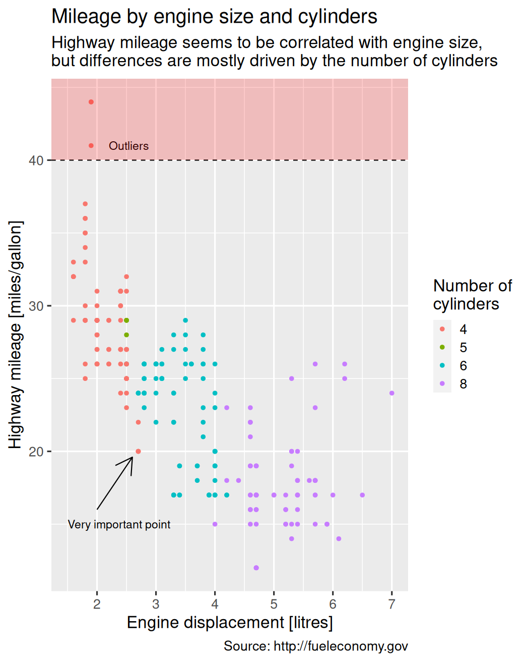
Types of Annotations
Types of Annotations
- Guides (axes and legend)
Types of Annotations
Guides (axes and legend)
Titles (title, subtitle and caption)
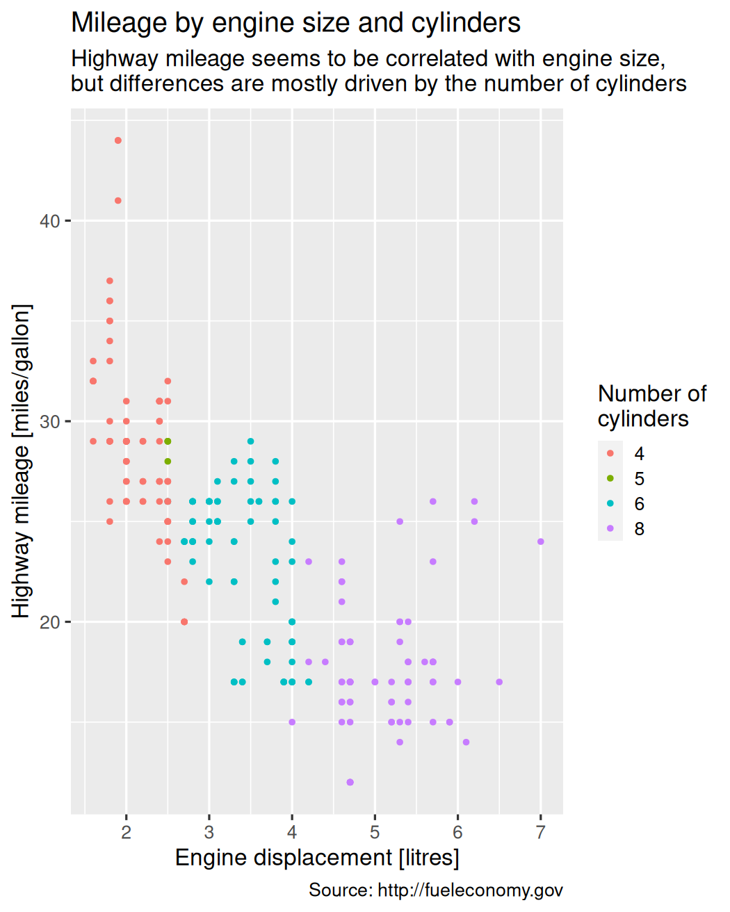
Types of Annotations
Guides (axes and legend)
Titles (title, subtitle and caption)
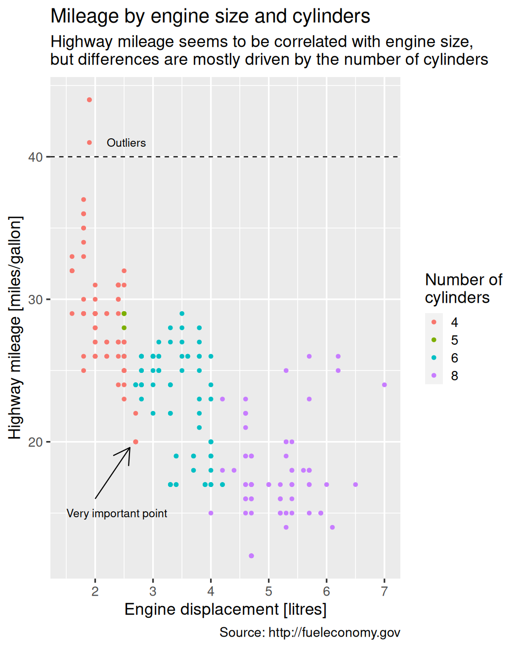
Text labels

Types of Annotations
Guides (axes and legend)
Titles (title, subtitle and caption)
Text labels
Reference lines
Types of Annotations
Guides (axes and legend)
Titles (title, subtitle and caption)
Text labels
Reference lines
Reference areas
Types of Annotations
Guides (axes and legend)
Titles (title, subtitle and caption)
Text labels
Reference lines
Reference areas
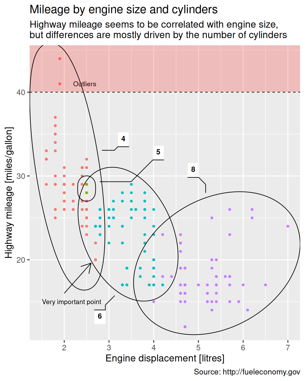
Direct labeling
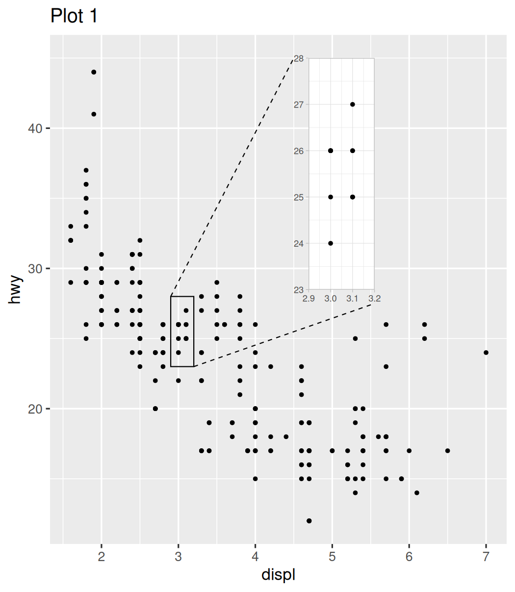
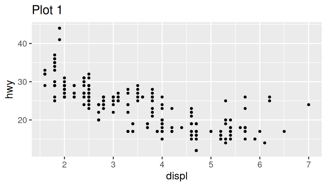
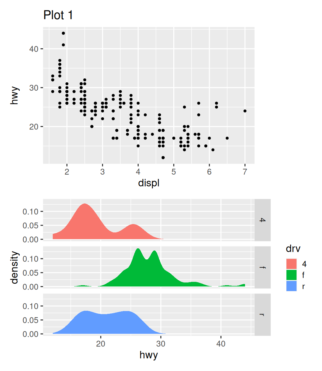
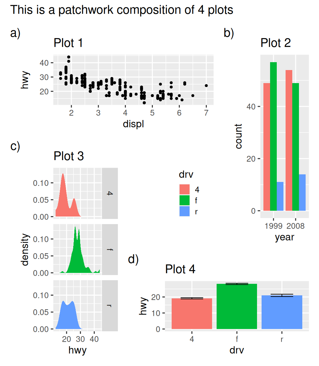
Types of Arrangements
- Compositions
- Insets